LEFT, RIGHT, and MID are among the first text functions most Excel users learn. They are simple, readable, and fast. They also break silently the moment the text they extract from changes its structure — and in real workbooks, text structures change constantly.
The failure mode is particularly dangerous because there is no error. The formula still runs and returns a result. The result is just wrong — off by a character, missing a digit, or picking up the wrong segment entirely. By the time someone notices, the corrupted data may already be in a report.
This post explains exactly why position-based extraction fails, shows you delimiter-based alternatives that adapt automatically, and introduces the modern functions that make all of this simpler.
The Exact Failure Mode
You receive a column of order codes in this format:
PRD-10234-US
PRD-845-US
PRD-120567-EU
You need to extract the numeric order number — the part between the two dashes. You write:
=MID(A2, 5, 5)This works for PRD-10234-US — position 5, length 5 gives you 10234. You copy it down the column and everything looks right.
Next month, a batch of short order numbers arrives:
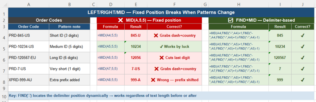
PRD-845-US   → MID(A,5,5) returns "845-U"  ← wrong
PRD-7-US     → MID(A,5,5) returns "7-US"   ← wrong
And a supplier starts using a longer prefix:
XPRD-999-AU → MID(A,5,5) returns "999-A" ← wrongNone of these return an error. All of them return something that looks like a valid value. The wrong data propagates downstream before anyone catches it.
Why Position-Based Extraction Is Fragile
LEFT, RIGHT, and MID all share one design assumption: the piece of text you want is always at a predictable character position. This assumption holds in controlled, system-generated data with strict formatting rules. It fails in almost any data that comes from humans, external vendors, or legacy systems.
Three things break positional assumptions in practice:
1. IDs and codes grow in length over time
Order numbers that started as three digits become four, then five. Customer IDs get a leading zero added for system compatibility. Product codes get a new category prefix. Every change shifts the character positions your formula depends on.
2. Optional segments appear or disappear
A country code suffix that was always two characters gets replaced with a three-character ISO code. A department prefix gets added to some records but not others. RIGHT and LEFT formulas assume the segment they target is always there and always the same length.
3. The error looks valid
A formula that returns "845-U" instead of "845" does not trigger any error checking. It is a valid text string. Downstream VLOOKUP formulas will simply fail to find a match — and you will spend time debugging the lookup rather than the extraction formula.
Delimiter-Based Extraction with FIND and MID
The solution is to anchor extraction to a delimiter — a character that separates the segments — rather than a character position. Delimiters like dashes, slashes, underscores, and dots are usually stable even when the content around them changes length.
Extract the segment between the first and second dash:
=MID(A2, FIND("-",A2)+1, FIND("-",A2,FIND("-",A2)+1) - FIND("-",A2) - 1)This formula works in three steps:
FIND("-",A2)finds the position of the first dashFIND("-",A2, FIND("-",A2)+1)finds the position of the second dash by starting the search after the first one- MID extracts everything between those two positions
For PRD-10234-US, PRD-845-US, and PRD-120567-EU, this formula returns 10234, 845, and 120567 respectively — correct in every case regardless of length.
Extract everything before the first dash:
=LEFT(A2, FIND("-",A2)-1)Extract everything after the last dash:
=RIGHT(A2, LEN(A2) - FIND("*", SUBSTITUTE(A2,"-","*", LEN(A2)-LEN(SUBSTITUTE(A2,"-","")))))The SUBSTITUTE trick replaces only the last occurrence of the dash with an asterisk, then FIND locates it. This is the standard all-version technique for finding the last delimiter.
Six Practical Extraction Patterns
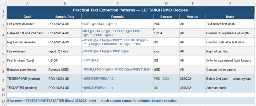
These patterns cover the most common real-world extraction tasks:
| Goal | Formula | Works on |
|---|---|---|
| Text before first delimiter | =LEFT(A2, FIND("-",A2)-1) | All versions |
| Text between 1st and 2nd delimiter | =MID(A2,FIND("-",A2)+1, FIND("-",A2,FIND("-",A2)+1)-FIND("-",A2)-1) | All versions |
| Text after last delimiter | =RIGHT(A2,LEN(A2)-FIND("*",SUBSTITUTE(A2,"-","*",LEN(A2)-LEN(SUBSTITUTE(A2,"-",""))))) | All versions |
| File extension | =RIGHT(A2, LEN(A2)-FIND(".",A2)) | All versions |
| Content inside parentheses | =MID(A2, FIND("(",A2)+1, FIND(")",A2)-FIND("(",A2)-1) | All versions |
| Fixed-length prefix (truly fixed) | =LEFT(A2, 2) | All versions |
Modern Alternatives: TEXTBEFORE, TEXTAFTER, TEXTSPLIT
Excel 365 and Excel 2021 introduced three functions that make delimiter-based extraction far cleaner:
TEXTBEFORE
=TEXTBEFORE(A2, "-")        ← everything before the first dash
=TEXTBEFORE(A2, "-", 2)     ← everything before the second dash
TEXTAFTER
=TEXTAFTER(A2, "-")         ← everything after the first dash
=TEXTAFTER(A2, "-", -1)     ← everything after the last dash
TEXTSPLIT
=TEXTSPLIT(A2, "-") ← splits into multiple columns: PRD | 10234 | USTEXTSPLIT spills results into adjacent cells automatically. It is the cleanest option when you need all segments extracted at once.

If you are on Excel 2019 or earlier, use the FIND-based patterns from the previous section. The results are identical — only the formula complexity differs.
When LEFT and RIGHT Are Still Fine
Position-based extraction is appropriate in a narrow set of situations where the format is genuinely fixed and guaranteed:
- File extensions of a known, enforced length (
.xlsxis always 4 characters) - Country codes with a guaranteed 2-character standard (ISO 3166-1 alpha-2)
- System-generated IDs with a contractual format specification that is unlikely to change
- Padded codes where all values are always the same total length
In all other cases — any data that originates from humans, external vendors, or systems you do not control — use delimiter-based formulas.
Comparison Table
| Method | Adapts to length changes? | All Excel versions? | Best for |
|---|---|---|---|
| LEFT(text, n) | No | Yes | Guaranteed fixed-length prefixes |
| RIGHT(text, n) | No | Yes | Guaranteed fixed-length suffixes |
| MID(text, s, n) | No | Yes | Guaranteed fixed-position middle |
| FIND + MID/LEFT/RIGHT | Yes | Yes | Variable-length, delimiter-based |
| TEXTBEFORE | Yes | 365/2021 only | Clean left extraction by delimiter |
| TEXTAFTER | Yes | 365/2021 only | Clean right extraction by delimiter |
| TEXTSPLIT | Yes | 365/2021 only | Split all segments at once |
| Flash Fill (Ctrl+E) | Yes (manual) | 2013+ | One-time cleanup, no formula needed |
Quick Checklist
- LEFT, RIGHT, and MID extract by character position — they break silently when text length changes
- The failure produces no error — just wrong values that look plausible
- Use FIND to locate delimiters dynamically instead of hardcoding positions
- The SUBSTITUTE trick finds the last occurrence of a delimiter in all Excel versions
- TEXTBEFORE and TEXTAFTER (Excel 365/2021) are cleaner alternatives to FIND-based formulas
- TEXTSPLIT splits a text string into multiple columns in one formula
- Reserve fixed-position LEFT and RIGHT for data with a contractually guaranteed format
- Test extraction formulas against short, long, and edge-case values before deploying
Frequently Asked Questions
Why does my MID formula return the wrong result for some rows?
MID extracts a fixed number of characters starting at a fixed position. When the text in those rows is shorter or longer than expected — a different number of digits in a code, an extra prefix, or a missing segment — the formula extracts from the wrong position. Replace the fixed start position and length with FIND-based expressions that locate the target segment relative to a delimiter, so the formula adapts to any length.
How do I extract text after the last delimiter in a cell?
In all Excel versions, use the SUBSTITUTE trick to find the last delimiter: =RIGHT(A2, LEN(A2)-FIND(“*”,SUBSTITUTE(A2,”-“,”*”,LEN(A2)-LEN(SUBSTITUTE(A2,”-“,””))))). This replaces only the last dash with an asterisk, then finds its position. In Excel 365 and 2021, the cleaner alternative is =TEXTAFTER(A2,”-“,-1), where -1 means the last occurrence.
What is Flash Fill and when should I use it?
Flash Fill (Ctrl+E, available in Excel 2013 and later) detects a pattern from a manually entered example and fills remaining cells. Type the desired extraction result for the first row, then press Ctrl+E. It is fast and requires no formula knowledge. However, it is a one-time operation — if new data arrives next month with a slightly different pattern, Flash Fill does not update automatically. Use Flash Fill for one-time cleanup tasks; use FIND-based formulas or TEXTBEFORE/TEXTAFTER for recurring data that may change.
Is TEXTBEFORE available in Excel 2019?
No. TEXTBEFORE, TEXTAFTER, and TEXTSPLIT are available only in Excel for Microsoft 365 and Excel 2021. They are not available in Excel 2019, 2016, or earlier. For those versions, use FIND combined with LEFT, RIGHT, or MID to achieve the same results — the formulas are longer but functionally equivalent.
How do I split a text column into multiple columns in Excel?
In Excel 365 and 2021, use TEXTSPLIT: =TEXTSPLIT(A2,”-“) splits the value by dash and spills results into adjacent cells automatically. In older versions, use Data → Text to Columns → Delimited, choose your delimiter, and Excel splits the column across multiple columns in one step. Text to Columns is a one-time operation; TEXTSPLIT updates automatically when the source changes.