You import a customer list. The IDs look identical to your master list. VLOOKUP returns #N/A for half of them. You manually retype one ID and suddenly the match works.
The data is not wrong. The cells contain invisible characters — spaces, line breaks, or control codes that travelled in with the import. Excel stores them as real content, which means every comparison, lookup, and deduplication fails for those rows, silently, with no error that points to the cause.
This post shows you how to detect hidden characters, which functions remove which kinds, and how to build a cleaning workflow that handles imported data reliably.
What Invisible Characters Do to Your Data
Invisible characters cause four categories of failure in Excel:
Lookups return #N/A
VLOOKUP, XLOOKUP, and MATCH compare values character by character. A customer ID of C-001 does not match C-001 (with a leading space) — they are different strings. The lookup returns #N/A even though both cells display identical text.
COUNTIF and COUNTIFS undercount
If your criteria range contains values with trailing spaces and your criteria do not, or vice versa, COUNTIF misses rows that visually match. The count appears lower than expected with no error to investigate. For more on this specific problem, see Why COUNTIF Returns 0 Even When Values Exist.
Duplicate removal misses matches
Remove Duplicates and UNIQUE treat Alice Kim and Alice Kim (trailing space) as two different values. Duplicates are not removed; unique lists contain near-duplicates that are invisible to the eye.
Sorting and grouping produce unexpected results
Values with leading spaces sort before values without them. Pivot Table grouping treats Seoul and Seoul as separate categories, splitting totals across two rows.
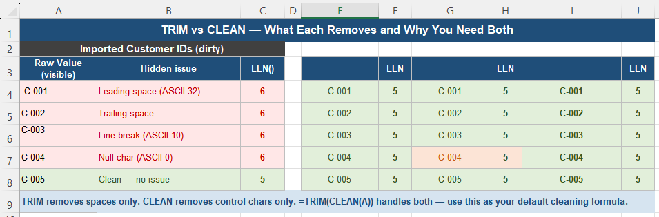
Where Hidden Characters Come From
Invisible characters almost never originate from manual typing. They arrive through:
- CSV and text file imports — line endings, BOM characters, and encoding artifacts
- Copy-paste from web pages or PDFs — non-breaking spaces (ASCII 160) are common in HTML
- ERP and database exports — fixed-width fields padded with trailing spaces
- Cross-platform files — Windows and Mac use different line ending characters
- Older Excel files — data cleaned for one system may contain characters meaningful only to that system
The pattern is consistent: data looks fine visually, but contains characters that Excel’s comparison engine treats as meaningful content.
How to Detect Hidden Characters
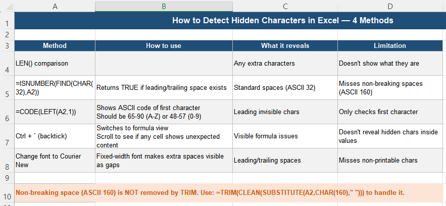
Method 1 — LEN comparison (most reliable)
=LEN(A2) - LEN(TRIM(CLEAN(A2)))If the result is greater than zero, the cell contains hidden characters. The number tells you how many were removed. Add this as a helper column when auditing imported data.
Method 2 — CODE of first character
=CODE(LEFT(A2,1))Returns the ASCII code of the first character. Normal letters return 65–90 (A–Z) or 97–122 (a–z). Numbers return 48–57. A return value of 32 means a leading space. Any value below 32 indicates a control character.
Method 3 — Fixed-width font
Change the column font to Courier New. In a fixed-width font, extra spaces become visually obvious as gaps before or after the text content.
Method 4 — Ctrl + ` (backtick)
Toggles formula view. While not directly revealing hidden characters, it helps identify cells where unexpected characters are embedded in formulas.
What TRIM Does (and Does Not Do)
TRIM removes leading spaces, trailing spaces, and reduces multiple consecutive spaces between words to a single space:
=TRIM(" Alice Kim ") → "Alice Kim"TRIM removes only standard spaces — ASCII character 32. It does not remove:
- Non-breaking spaces (ASCII 160, common in web copy-paste)
- Control characters (ASCII 0–31, common in database exports)
- Tab characters (ASCII 9)
If your data contains only extra spaces from manual entry or copy-paste of normal text, TRIM alone is sufficient. For anything imported from external systems, combine it with CLEAN.
What CLEAN Does (and Does Not Do)
CLEAN removes non-printable characters — ASCII codes 0 through 31. These include line breaks (ASCII 10), carriage returns (ASCII 13), null characters (ASCII 0), and tab characters (ASCII 9):
=CLEAN("C-003" & CHAR(10)) → "C-003" (line break removed)CLEAN does not remove:
- Standard spaces (ASCII 32) — that is TRIM’s job
- Non-breaking spaces (ASCII 160) — these are printable characters, above ASCII 31
The Standard Fix: TRIM(CLEAN())
For most imported data, wrapping CLEAN inside TRIM handles the full range of common hidden characters:
=TRIM(CLEAN(A2))CLEAN runs first, removing control characters. TRIM then removes any spaces that remain, including those that were adjacent to the removed control characters. This combination handles 90% of real-world cleaning scenarios.
Apply it in a helper column — never directly on the raw data column:
Column A: raw imported value (untouched)
Column B: =TRIM(CLEAN(A2))   ← use this column in all downstream formulas
Handling Non-Breaking Spaces
Non-breaking spaces (ASCII 160) are used in HTML to prevent line breaks. When you copy text from a web page, they travel with the content. Neither TRIM nor CLEAN removes them.
Detect them with:
=ISNUMBER(FIND(CHAR(160), A2)) → TRUE if non-breaking space is presentRemove them with SUBSTITUTE before applying TRIM and CLEAN:
=TRIM(CLEAN(SUBSTITUTE(A2, CHAR(160), " ")))SUBSTITUTE replaces each non-breaking space with a standard space, then TRIM removes the resulting extra spaces.
For data copied from web pages or email, this three-function combination is the complete solution:
=TRIM(CLEAN(SUBSTITUTE(A2, CHAR(160), " ")))Safe Cleaning Workflow
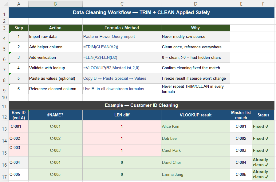
Follow this sequence when working with imported data:
- Keep the raw column untouched. Never apply cleaning formulas directly to the imported data. You need the original for validation and rollback.
- Create a helper column with =TRIM(CLEAN(A2)). Fill it down for all rows.
- Add a verification column: =LEN(A2)-LEN(B2). Any non-zero value confirms hidden characters were present and removed.
- Test your lookups against the cleaned column. If matches that previously failed now work, the cleaning resolved the problem.
- Reference the cleaned column in all downstream formulas — VLOOKUP, COUNTIF, SUMIFS, and so on. Never repeat TRIM(CLEAN()) inside every formula; centralize it once.
- Paste as values only when the source will not change. If new data arrives weekly, keep the formula active so it cleans automatically.
Quick Checklist
- Lookups failing on visually identical values → hidden characters are the most common cause
- Use =LEN(A2)-LEN(TRIM(CLEAN(A2))) to detect hidden characters — any non-zero result means they exist
- TRIM removes extra spaces (ASCII 32) only
- CLEAN removes control characters (ASCII 0–31) only
- =TRIM(CLEAN(A2)) handles both — use this as the default cleaning formula
- Non-breaking spaces (ASCII 160) require SUBSTITUTE(A2,CHAR(160),” “) before TRIM and CLEAN
- Always clean in a helper column — never overwrite the raw import
- Reference the cleaned column everywhere; never repeat cleaning logic inside lookup formulas
Frequently Asked Questions
Why does VLOOKUP return #N/A when the values look identical?
The most common cause is hidden characters — usually a leading or trailing space, a line break, or a non-breaking space — in either the lookup value or the lookup range. VLOOKUP compares strings exactly, character by character. “C-001″ and ” C-001″ (with a leading space) are different strings. Apply =TRIM(CLEAN()) to both the lookup value and the lookup range, then retry. If the match succeeds, hidden characters were the cause.
What is the difference between TRIM and CLEAN in Excel?
TRIM removes leading spaces, trailing spaces, and reduces multiple consecutive spaces between words to one. It only handles ASCII 32 (the standard space character). CLEAN removes non-printable control characters — ASCII codes 0 through 31 — including line breaks, carriage returns, and null characters. It does not remove spaces. For imported data, use both together: =TRIM(CLEAN(A2)).
Why doesn’t TRIM remove the space in my imported data?
The space is likely a non-breaking space (ASCII 160), not a standard space (ASCII 32). TRIM only removes ASCII 32. Non-breaking spaces are common in data copied from web pages or HTML-based systems. Remove them with: =TRIM(CLEAN(SUBSTITUTE(A2, CHAR(160), ” “))). This replaces non-breaking spaces with standard spaces first, then TRIM removes them.
Is it safe to apply TRIM and CLEAN directly to the original data?
It is generally not recommended. Apply cleaning in a helper column and keep the original data untouched. This lets you verify that cleaning worked correctly by comparing the two columns, roll back if the formula removes something it should not have, and understand what the raw data looked like if questions arise later. Once you have confirmed the cleaning is correct, you can paste the cleaned values over the original if needed.
How do I check whether a cell contains a non-breaking space?
Use =ISNUMBER(FIND(CHAR(160),A2)). This returns TRUE if a non-breaking space (ASCII 160) is present in the cell. Alternatively, compare LEN(A2) with LEN(TRIM(CLEAN(SUBSTITUTE(A2,CHAR(160),” “)))) — if the numbers differ after the full cleaning formula, the cell contained hidden characters including non-breaking spaces.