Your COUNTIF formula should return 4. It returns 2. You check the data — every cell looks like it says “Seoul.” But some of them say “Seoul” and others say ” Seoul” or “Seoul ” — with an invisible leading or trailing space. Excel’s comparison engine sees them as completely different strings, and your conditions silently fail for the rows that have the extra space.
This is one of the most common data quality issues in Excel, almost always introduced through imports, and almost never visible on screen. This post walks through why this happens, shows you how to detect which rows are affected, and gives you the methods that fix it reliably.
How Extra Spaces Break Conditions
Excel’s comparison logic is exact: "Seoul" equals "Seoul" and nothing else. A value with a leading space — " Seoul" — is a different string, and Excel treats it as such in every IF, COUNTIF, SUMIF, VLOOKUP, and MATCH formula. The comparison fails for that row, and the failure produces no error, no warning, and no visible difference in the cell display.
Four Reasons This Keeps Happening
1. Spaces are invisible by default
A cell containing " Seoul" looks identical to a cell containing "Seoul" in a standard spreadsheet view. There is no visual indication that extra characters are present, and the default left-aligned text display provides no spatial clue about leading spaces.
2. Imported data frequently includes trailing spaces from fixed-width fields
ERP systems, database exports, and CSV files from legacy systems often pad text fields to a fixed width with trailing spaces — a formatting convention from older systems that has no meaning in Excel but travels with the data faithfully.
3. Copy-paste from web pages introduces non-breaking spaces
Web content uses non-breaking spaces (ASCII 160) in addition to regular spaces (ASCII 32). Both look identical on screen, but TRIM only removes ASCII 32 spaces, leaving ASCII 160 intact. This means a TRIM-based fix may appear to work without actually resolving every case.
4. Multiple spaces can appear inside values, not just at the edges
TRIM removes leading, trailing, and multiple consecutive internal spaces — but only standard ASCII 32 spaces. Internal spaces that are intentional (a single space between words) are preserved, while extra duplicates are removed. This behavior is correct, but it means TRIM is not a simple “remove all spaces” function.
Scenario: A Regional Sales Filter
Consider an imported sales table where the Region column appears to contain only “Seoul” and “Busan.” A COUNTIF for “Seoul” returns 2 when there are clearly 4 Seoul rows visible on screen, and SUMIF similarly understates the Seoul total.

Detecting Which Rows Are Affected
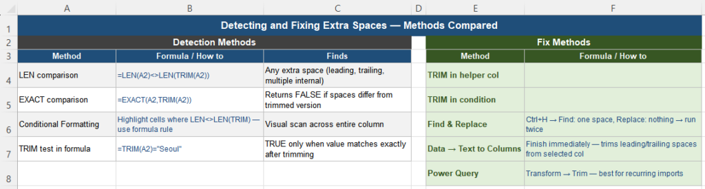
Before fixing, confirm exactly which rows contain extra spaces. Three methods work reliably:
Method 1 — LEN comparison
=LEN(A2) <> LEN(TRIM(A2))Returns TRUE for any cell where the length differs after trimming — meaning extra spaces exist. Add this as a helper column and filter for TRUE rows to see exactly which cells are affected.
Method 2 — EXACT comparison
=EXACT(A2, TRIM(A2))Returns FALSE when the cell’s value does not exactly match its trimmed version. EXACT is case-sensitive and character-sensitive, making it more reliable than a plain = comparison for this purpose.
Method 3 — Conditional Formatting
Apply a Conditional Formatting rule using the formula =LEN(A1)<>LEN(TRIM(A1)) across the column. This highlights affected cells immediately in a visual scan, without adding helper columns.
Fixing the Problem
Option 1 — TRIM in a helper column (recommended for recurring data)
=TRIM(A2)Apply this in an adjacent column for every row, then reference the cleaned column in all COUNTIF, SUMIF, and IF formulas rather than the original. The raw column stays intact for reference and audit, and the cleaning logic runs automatically for every new row appended to the dataset.
Option 2 — TRIM inside the condition formula
For a one-off fix where adding a helper column is impractical, TRIM can be embedded directly inside the counting formula using SUMPRODUCT:
=SUMPRODUCT((TRIM(A2:A100)="Seoul")*1)This applies TRIM to every cell at evaluation time and counts matches against the trimmed values. It is slower on large ranges than a pre-cleaned helper column, but eliminates the need for any structural change to the sheet.
Option 3 — Find & Replace (one-time cleanup)
Press Ctrl + H, enter a single space in the Find field and leave Replace blank, then click Replace All. Run it twice — once may not catch double spaces completely. This modifies the source data directly, so only use it when the raw import is no longer needed for reference.
Option 4 — Data → Text to Columns (one-time cleanup)
Select the column, go to Data → Text to Columns, choose Delimited, click Next without selecting any delimiter, then click Finish. This operation trims leading and trailing spaces from the selected column as a side effect, without splitting any values. Like Find & Replace, it modifies the source directly.
Option 5 — Non-breaking spaces require SUBSTITUTE
If TRIM does not resolve all cases, the remaining cells likely contain non-breaking spaces (ASCII 160). Handle these with an additional SUBSTITUTE step:
=TRIM(SUBSTITUTE(A2, CHAR(160), " "))This replaces non-breaking spaces with regular spaces first, then TRIM removes them along with any standard leading or trailing spaces.
Prevent It From Recurring
Fixing spaces in the current import is useful. Preventing the same problem from appearing in next month’s import is better. Two habits address this structurally:
Build the TRIM layer before the data is used. As soon as data is imported, apply =TRIM(A2) in a dedicated cleaning column before any COUNTIF, SUMIF, or VLOOKUP formula references the data. This way, even if the next import contains the same space issues, the cleaning step already handles them automatically.
For recurring imports, use Power Query. Power Query’s Transform → Trim operation applies a consistent, repeatable cleaning step that runs every time the query is refreshed, before any data reaches the Excel sheet. This is the most reliable approach for data that arrives regularly from the same source with the same formatting issues.
Separate Raw Data From Clean Data
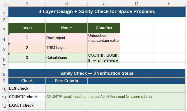
| Layer | Name | Contains |
|---|---|---|
| 1 | Raw Import | Untouched — may contain extra spaces |
| 2 | TRIM Layer | =TRIM(A2) applied once — this column is used everywhere downstream |
| 3 | Calculations | COUNTIF, SUMIF, IF — all reference Layer 2, never Layer 1 directly |
Quick Checklist
- A single extra space makes “Seoul” and ” Seoul” different strings — conditions fail silently
- Use =LEN(A2)<>LEN(TRIM(A2)) to identify which rows contain extra spaces
- TRIM in a helper column is the recommended structural fix for recurring data
- SUMPRODUCT with TRIM inside the condition works for one-off fixes without a helper column
- Find & Replace and Text to Columns are faster but modify source data directly
- Non-breaking spaces (ASCII 160) require SUBSTITUTE(A2,CHAR(160),” “) before TRIM
- Build the TRIM layer before any formula references the imported data
- For regular imports, apply TRIM in Power Query to prevent the problem from recurring automatically
Frequently Asked Questions
Why does COUNTIF return a lower number than expected even when the values look identical?
Some cells likely contain extra spaces — leading, trailing, or both — that are invisible in the standard cell display. Excel’s comparison logic is exact: “Seoul” with a leading space is a different string from “Seoul” without one, so COUNTIF misses those rows. Use =LEN(A2)<>LEN(TRIM(A2)) in a helper column to identify which rows are affected, then apply TRIM to the source column or use SUMPRODUCT with TRIM inside the condition formula.
What does TRIM actually do — does it remove all spaces?
TRIM removes leading spaces, trailing spaces, and reduces any sequence of multiple consecutive spaces between words to a single space. It only affects standard spaces (ASCII 32). It does not remove non-breaking spaces (ASCII 160, common in web copy-paste), tab characters, or other whitespace characters. For non-breaking spaces, use SUBSTITUTE(A2,CHAR(160),” “) before TRIM to convert them to regular spaces first.
How can I use COUNTIF without adding a helper column?
Use SUMPRODUCT with TRIM applied inside the condition: =SUMPRODUCT((TRIM(A2:A100)=”Seoul”)*1). This applies TRIM to each cell at evaluation time and counts the matches against the trimmed values. It is slower than a pre-cleaned helper column on large datasets but eliminates any structural change to the sheet. For SUMIF equivalents, use =SUMPRODUCT((TRIM(A2:A100)=”Seoul”)*B2:B100).
Why does TRIM not fix the spaces in some of my cells?
The remaining cells likely contain non-breaking spaces (ASCII 160) rather than standard spaces (ASCII 32). TRIM only removes ASCII 32. To handle non-breaking spaces, use =TRIM(SUBSTITUTE(A2,CHAR(160),” “)) — this converts non-breaking spaces to regular spaces first, then TRIM removes them. Verify with =ISNUMBER(FIND(CHAR(160),A2)) to confirm whether non-breaking spaces are present.
Is it safe to use Find and Replace to remove spaces from a data column?
Find and Replace modifies the source data directly and cannot be undone after saving. It is safe for a one-time cleanup when you no longer need the original values for reference, but it is not appropriate for recurring imports or any situation where the original data may need to be audited later. For recurring data, use a TRIM helper column that keeps the raw import intact while providing clean values for all downstream formulas.
Related Articles
Why COUNTIF Returns 0 Even When Values Exist