You apply a filter, copy the visible rows, and paste them into a summary sheet. It looks correct — until the source data changes and the pasted copy quietly stops reflecting reality.
This is not a filtering problem. It is a snapshot problem. AutoFilter only hides rows visually; the moment you copy what’s visible, you capture a frozen picture, not a rule. FILTER replaces that picture with a live formula that re-extracts matching rows every time the data changes.
This post explains why manual filtering creates this gap, walks through building a self-updating FILTER-based view, and shows you the condition patterns used most often in real reports.
Why Copied Filter Results Go Stale
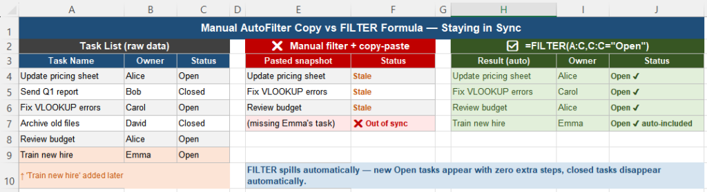
Consider a task list with Task Name, Owner, and Status columns. You need a separate view showing only tasks where Status equals “Open,” refreshed daily for a team standup.
The manual approach: apply AutoFilter on the Status column, set it to “Open,” copy the visible rows, and paste them into a summary area. This works for the data that exists at that moment.
The next day, a new task is added with Status “Open.” The raw data updates. The pasted summary does not — it still shows yesterday’s filtered set, missing the new task entirely, with no indication that anything is out of date.
Four Reasons This Keeps Happening
1. Manual filters create views, not logic
AutoFilter hides rows visually — it does not change the underlying data, and it does not store the condition anywhere reusable. Copying the visible rows captures only the result of that one moment, with no connection back to the rule that produced it.
2. Older formulas were not row-aware
Traditional Excel formulas return one value per cell. There was no native way to ask a formula to “return all rows where Status equals Open” — that required AutoFilter, Advanced Filter, or VBA. This pushed extraction work toward manual, one-time operations.
3. Real reports depend on conditional subsets constantly
Office work is full of recurring subset needs: only this month’s transactions, only active customers, only tasks assigned to a specific team. When each of these subsets is built manually, they all drift independently as the source data evolves.
4. FILTER changes the extraction model entirely
FILTER does not hide rows from a table — it creates a new table based on a condition and keeps that table live. This is a structural shift from “view of existing data” to “formula-generated data,” and it is what eliminates the staleness problem.
Building a Live FILTER View Step by Step
Step 1 — Point FILTER directly at the source. Assuming task data occupies columns A through C with Status in column C:
=FILTER(A:C, C:C="Open")This returns all columns, but only for rows where Status equals “Open.” There is no copying and no hidden rows — the result is generated fresh from the current data every time it recalculates.
Step 2 — Let the result spill naturally. The output expands when new matching rows appear and shrinks when rows no longer match. Do not try to constrain it with a fixed range — the spill behavior is the entire point.
Step 3 — Handle the empty-result case. If no rows match the condition, FILTER returns a #CALC! error. Wrap it once:
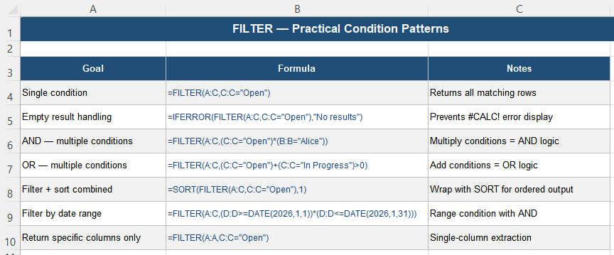
=IFERROR(FILTER(A:C, C:C="Open"), "No results")This produces clean output instead of a visible error when the filtered set happens to be empty.
Step 4 — Use the extracted table downstream. Base charts, summaries, or further calculations on the FILTER output rather than the raw data. This keeps the extraction logic in one place — every dependent element stays in sync automatically.
Sanity check: add a new task marked “Open.” It should appear in the FILTER output instantly. Change an existing task’s status away from “Open.” It should disappear. If both happen without touching any formula, the extraction is genuinely live.
AND, OR, and Combined Condition Patterns
Single condition:
=FILTER(A:C, C:C="Open")AND — multiple conditions must all be true:
=FILTER(A:C, (C:C="Open")*(B:B="Alice"))Multiplying condition arrays produces AND logic — a row is included only if both conditions evaluate to TRUE (1).
OR — at least one condition must be true:
=FILTER(A:C, (C:C="Open")+(C:C="In Progress")>0)Adding condition arrays produces OR logic. The >0 check ensures a row is included if either condition is true, without double-counting. This is the same pattern used for OR logic in SUMPRODUCT — see Why OR Conditions Don’t Work as Expected in Excel Formulas for more on this technique.
Filter and sort together:
=SORT(FILTER(A:C, C:C="Open"), 1)Date range condition:
=FILTER(A:C, (D:D>=DATE(2026,1,1))*(D:D<=DATE(2026,1,31)))Where FILTER Belongs in Your Workbook
Stable workbooks separate data into three layers, and FILTER belongs specifically in the middle one:
| Layer | Name | Contains |
|---|---|---|
| 1 | Raw Data | Unchanged source data — never filtered or modified directly |
| 2 | FILTER Views | Live, condition-based extractions referencing layer 1 |
| 3 | Reports & Summaries | Charts and dashboards referencing layer 2 output |
This separation means the extraction logic exists in exactly one place. If the condition needs to change — for example, adding “In Progress” to the Open filter — you update one FILTER formula, and every chart and summary built on it updates automatically.
FILTER vs Pivot Table
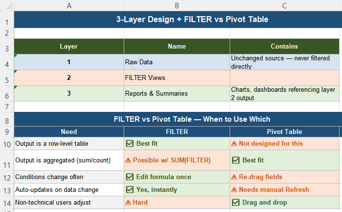
| Need | FILTER | Pivot Table |
|---|---|---|
| Output is a row-level table | Best fit | Not designed for this |
| Output is aggregated (sum, count) | Possible but indirect | Best fit |
| Conditions change frequently | Edit the formula once | Re-drag fields manually |
| Auto-updates when data changes | Yes, instantly | Requires manual Refresh |
| Non-technical users adjust filters | Harder — formula-based | Easy — drag and drop |
Use FILTER when the output needs to be a live table of matching rows. Use a Pivot Table when the output is a summary or aggregation and the audience needs to adjust filters themselves without editing formulas.
Quick Checklist
- AutoFilter hides rows visually but does not change or remember the underlying condition
- Copying filtered rows captures a snapshot that goes stale as soon as source data changes
=FILTER(range, condition)creates a live, condition-based table that updates automatically- Wrap FILTER in IFERROR to handle the case where no rows match
- Multiply conditions for AND logic; add conditions for OR logic
- Keep FILTER formulas in a dedicated layer between raw data and final reports
- Use Pivot Tables instead of FILTER when the goal is aggregation, not a row-level table
- Test by adding a new matching row and changing an existing row’s condition — both should update instantly
Frequently Asked Questions
Why does my filtered report not show new rows that match the condition?
If the report was built by applying AutoFilter and copying the visible rows, the result is a static snapshot with no connection to the source data. New matching rows added afterward will never appear unless you repeat the filter-and-copy process. Replace the copied range with a FILTER formula such as =FILTER(A:C, C:C=”Open”), which recalculates automatically whenever the source data changes.
Why does FILTER return a #CALC! error?
FILTER returns #CALC! when no rows in the source range match the specified condition. This is expected behavior, not a formula mistake. Wrap the FILTER formula in IFERROR to display a clean message instead: =IFERROR(FILTER(A:C,C:C=”Open”), “No results”). This prevents the error from appearing in a report while still correctly reflecting that no rows currently match.
How do I filter on multiple conditions at the same time?
For AND logic — where all conditions must be true — multiply the condition arrays together: =FILTER(A:C, (C:C=”Open”)*(B:B=”Alice”)). For OR logic — where at least one condition must be true — add the condition arrays and check for a result greater than zero: =FILTER(A:C, (C:C=”Open”)+(C:C=”In Progress”)>0). This is the same array-math approach used in SUMPRODUCT for combining conditions.
Should I use FILTER or a Pivot Table for my report?
Use FILTER when you need a live, row-level table of records matching specific conditions — for example, a list of open tasks. Use a Pivot Table when you need aggregated summaries — totals, counts, or averages grouped by category. FILTER updates instantly when source data changes; Pivot Tables require a manual Refresh. If your audience needs to adjust filters themselves without touching formulas, a Pivot Table’s drag-and-drop interface is easier for non-technical users.
Is FILTER available in Excel 2019?
No. FILTER is available only in Excel for Microsoft 365 and Excel 2021. It is not available in Excel 2019, 2016, or earlier. For those versions, use Advanced Filter (Data tab → Sort & Filter → Advanced) to extract matching rows to a new location, though this requires manually re-running the operation whenever the source data changes — it does not update automatically the way FILTER does.