You build a clean list of customer names: no duplicates, sorted alphabetically. It looks perfect. Next week, new transactions come in — and the list you built is already wrong. Nobody changed it. The data simply moved on without it.
This is the defining weakness of manual list-building in Excel: copy, deduplicate, and sort produce a snapshot, not a rule. The moment the source data changes, the snapshot goes stale, and someone has to notice and redo the entire process.
UNIQUE and SORT solve this by replacing the snapshot with a live formula. This post explains why manual lists break down, how dynamic array functions work differently, and how to build dropdowns, summaries, and reports that update themselves automatically.
Why Manual Lists Go Stale
Consider a transaction table with a Customer Name column. You need a separate list: one row per customer, sorted alphabetically, used to populate a dropdown and a summary sheet.
The manual approach: copy the Customer Name column, paste it elsewhere, run Remove Duplicates, then sort alphabetically. This works — for the data that exists at that exact moment.
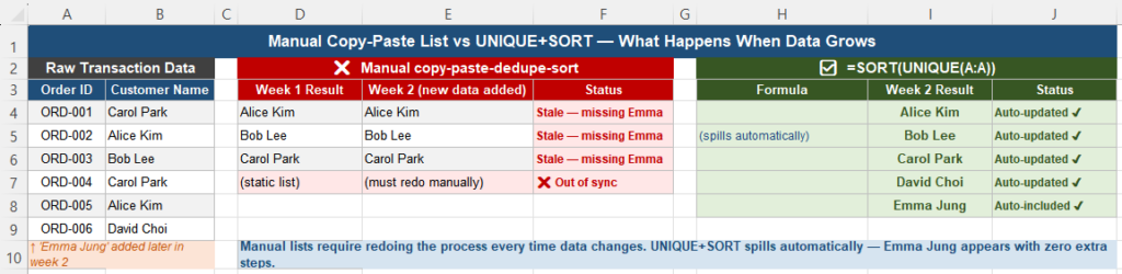
The following week, three new transactions arrive, one from a new customer. The transaction table updates automatically. The customer list does not. It still shows last week’s customers, missing the new one, and nothing about the spreadsheet indicates this has happened.
Four Reasons This Keeps Happening
1. Manual lists are snapshots, not logic
When you copy data and remove duplicates by hand, Excel stores the result of that one operation — not a rule that says “always show unique customers.” There is no connection between the list and its source after the operation completes.
2. Traditional formulas were not designed for lists
Classic Excel formulas operate on a one-formula-to-one-cell model. There was no native function that could return a deduplicated, sorted list of unbounded size. This pushed users toward manual processes that worked but did not scale.
3. Failures happen at the edges, not the center
The core data and main calculations in a report are usually correct. The failures appear in supporting elements — dropdown sources, summary headers, category lists — which depend on clean, current lists and are the easiest pieces to forget when data changes.
4. Dynamic array functions changed the underlying model
UNIQUE and SORT do not return a single value into a single cell. They return a live array that spills into as many cells as needed and automatically expands or contracts as the source data changes. This is a fundamentally different model from cell-by-cell formulas, and it is what makes self-updating lists possible.
Building a Self-Updating List Step by Step
Step 1 — Reference the raw data directly. Do not pre-clean the list manually. Point the formula at the source column itself, so new and removed entries are reflected automatically.
Step 2 — Generate the unique list:
=UNIQUE(A:A)Excel spills the result downward into as many cells as there are unique values. Duplicates are removed, and the result resizes automatically as data changes.
Step 3 — Add sorting on top:
=SORT(UNIQUE(A:A))This single formula replaces the entire copy, paste, deduplicate, and sort sequence. One row per customer, alphabetically ordered, with zero manual steps.
Step 4 — Reference the spilled range downstream. Use the spill reference operator # rather than a hardcoded range:
=COUNTA(D1#)        ← counts all values in the spilled list, however many there are
=SORT(UNIQUE(A:A))   in D1, then D1# always refers to the current spill
Never hardcode the range size (such as D1:D50) for a list that grows. If the source data grows beyond your hardcoded range, the downstream formula misses the new entries — the exact problem this approach is meant to solve.
Sanity check: add a new row to the raw data. The list should expand immediately, the sort order should remain correct, and no formulas should need editing. If this happens, the setup is stable.
Practical UNIQUE and SORT Patterns
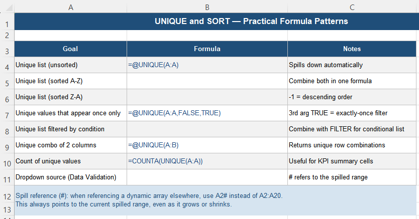
| Goal | Formula |
|---|---|
| Unique list (unsorted) | =UNIQUE(A:A) |
| Unique list, sorted A-Z | =SORT(UNIQUE(A:A)) |
| Unique list, sorted Z-A | =SORT(UNIQUE(A:A),1,-1) |
| Values that appear exactly once | =UNIQUE(A:A,FALSE,TRUE) |
| Unique list filtered by condition | =SORT(UNIQUE(FILTER(A:A,B:B="Seoul"))) |
| Unique combinations of two columns | =UNIQUE(A:B) |
| Count of unique values (KPI cell) | =COUNTA(UNIQUE(A:A)) |
For conditional unique lists — for example, unique customers from only the Seoul region — combining UNIQUE with FILTER lets you build the entire pipeline in one formula. For more on FILTER, see Why Conditional Data Extraction Breaks in Excel Reports.
Self-Updating Dropdown Lists
One of the most useful applications of UNIQUE is a dropdown that updates itself as new categories are added to the source data.
- Place raw data in column A — never pre-clean it manually.
- In a helper cell (for example, D1), enter
=SORT(UNIQUE(A2:A1000)). - Select the target cell where you want the dropdown, then go to the Data tab → Data Validation.
- Set Allow to “List” and enter
=$D$1#as the source — the spill reference, not a fixed range. - Click OK. The dropdown now includes every current unique value and updates automatically as the source grows.

Version Compatibility
UNIQUE, SORT, FILTER, and the spill reference operator are available only in Excel for Microsoft 365 and Excel 2021. They do not work in Excel 2019, 2016, or earlier.
| Function | 365 / 2021 | 2019 / 2016 | Alternative for older versions |
|---|---|---|---|
| UNIQUE | Yes | No | Remove Duplicates (manual) or Pivot Table |
| SORT | Yes | No | Data → Sort (manual) |
| FILTER | Yes | No | AutoFilter or Advanced Filter |
| Spill reference (#) | Yes | No | Named range combined with OFFSET and COUNTA |
If your workbook must support Excel 2019 or earlier, a Pivot Table is the most practical substitute for a self-updating unique list — it can be set to refresh automatically on file open, which approximates the same outcome with one extra click.
Quick Checklist
- Manual copy-paste-deduplicate-sort produces a snapshot that goes stale as soon as new data arrives
=UNIQUE(A:A)returns a live, auto-resizing list of distinct values=SORT(UNIQUE(A:A))combines deduplication and sorting in a single formula- Reference spilled arrays with the
#operator — never hardcode the output range - Combine UNIQUE with FILTER for conditional unique lists
- Use the spill reference as the source in Data Validation for self-updating dropdowns
- UNIQUE, SORT, FILTER, and the spill operator require Excel 365 or 2021 — use Pivot Tables in older versions
- If you find yourself repeating manual deduplication regularly, that repetition is the signal to switch to UNIQUE
Frequently Asked Questions
Why does my deduplicated list go out of date?
Manual deduplication using Remove Duplicates or copy-paste creates a static snapshot of the data at the moment you ran it. It has no ongoing connection to the source data. When new rows are added later, the deduplicated list does not update — it simply reflects what existed when you last ran the process. Replace it with =UNIQUE(A:A), which recalculates automatically whenever the source data changes.
What is the difference between UNIQUE and Remove Duplicates?
Remove Duplicates is a one-time manual operation that deletes duplicate rows from the data itself — it modifies your data and must be re-run whenever new duplicates appear. UNIQUE is a formula that returns a live list of distinct values without modifying the original data. The UNIQUE result updates automatically every time the source range changes, with no manual steps required.
What does the # symbol mean in an Excel formula?
The # symbol is the spill reference operator. If cell D1 contains a dynamic array formula like =SORT(UNIQUE(A:A)) that spills into D1, D2, D3, and so on, then D1# refers to the entire spilled range — however many cells it currently occupies. This is different from a fixed range like D1:D50, which does not adjust if the spill grows or shrinks.
Can I use UNIQUE and SORT in Excel 2019?
No. UNIQUE, SORT, FILTER, and the spill reference operator are available only in Excel for Microsoft 365 and Excel 2021. They are not available in Excel 2019, 2016, or earlier versions. For those versions, use a Pivot Table set to refresh on file open as the closest equivalent, or continue using manual Remove Duplicates and Sort, accepting that the result will need to be re-run when data changes.
How do I make a dropdown list that updates automatically?
Create a helper cell with =SORT(UNIQUE(YourRange)). Then, in Data Validation (Data tab → Data Validation → Allow: List), set the source to the spill reference of that cell, such as =$D$1#. This causes the dropdown to automatically include any new unique values added to the source range, without needing to edit the dropdown’s source range manually.