You write a VLOOKUP formula. It works. A week later, a colleague inserts a new column into the table — and your formula starts returning the wrong values without any warning.
No #REF! error. No #VALUE!. Just quietly incorrect data flowing into your report.
This is one of the most dangerous failure modes in Excel, because the formula looks fine. The numbers look plausible. And you only find out something is wrong when a decision has already been made on bad data.
This post explains exactly why VLOOKUP behaves this way, shows you three formulas that do not have this problem, and gives you a step-by-step plan for replacing VLOOKUP in existing workbooks.
The Exact Scenario Where VLOOKUP Breaks
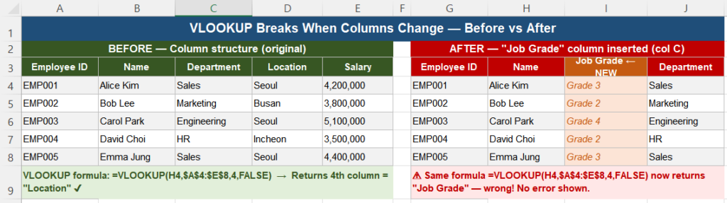
Here is the scenario in its simplest form:
- Your table has five columns: Employee ID, Name, Department, Location, Salary.
- You write
=VLOOKUP(A2, $B:$F, 3, FALSE)to return the Department — the 3rd column in the range. - A colleague inserts a new “Job Grade” column between Name and Department.
- Your formula still runs without errors — but now returns Job Grade instead of Department.
The formula did exactly what it was told: return whatever is in the 3rd column. The problem is that the 3rd column is now something different than it was when the formula was written.
Why This Happens — The Column Index Problem
VLOOKUP’s third argument is a column index number — a hardcoded integer that tells Excel which column to return, counted from the left edge of the lookup range.
The critical word is hardcoded. When you write 3, Excel stores the number 3. It does not store “the Department column.” It has no memory of your intention — only the position you specified at the time of writing.
Every structural change to the table — insert, delete, move, or reorder a column — shifts those positions. The number 3 now points somewhere new, but the formula has no way to detect this.
This is not a bug in Excel. VLOOKUP is working exactly as designed. The design assumption was that tables stay structurally stable. In real workbooks used by real teams, that assumption is almost never true for long.
Why the Error Is Silent
If VLOOKUP’s column index pointed outside the lookup range, you would get a #REF! error — visible and easy to catch. But in the scenario above, the index still points to a valid column. It just points to the wrong one.
Excel has no way to distinguish “the column I intended” from “a column that happens to be in this position.” From Excel’s perspective, the formula is working correctly.
This is why column-shift errors are more dangerous than formula errors. A formula that returns #N/A gets attention immediately. A formula that returns a plausible-looking wrong value gets copy-pasted into reports and acted upon.
The only way to detect this class of error is to manually verify that the column index still points to the right column after every structural change — which is not realistic in a collaborative workbook.
Three Formulas That Survive Column Changes
Option 1 — INDEX/MATCH (works in all Excel versions)
INDEX/MATCH replaces the column index number with a direct column reference. Instead of saying “return the 3rd column,” it says “return values from the Department column.”
VLOOKUP (fragile):
=VLOOKUP(A2, $B:$F, 3, FALSE)INDEX/MATCH (robust):
=INDEX(D:D, MATCH(A2, $A:$A, 0))How to read this formula: MATCH finds the row where A2 appears in column A. INDEX returns the value from that same row in column D (Department). If Department moves from column D to column E, you update one reference — or better yet, use a named column so nothing needs updating at all.
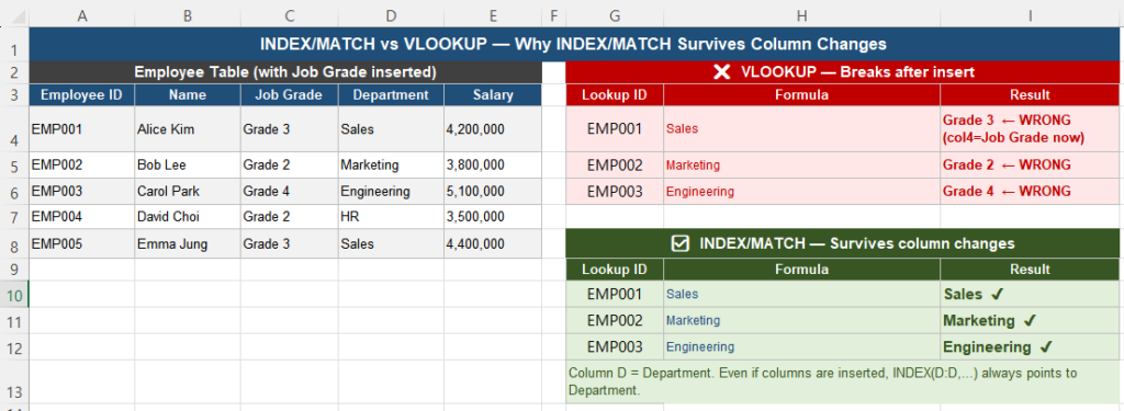
The 0 at the end of MATCH is critical — it forces exact match. Never omit it.
Option 2 — INDEX/MATCH with Excel Table references
If your data is in an Excel Table (created with Ctrl+T), you can reference columns by name instead of by letter:
=INDEX(Employees[Department], MATCH(A2, Employees[Employee ID], 0))Now the formula is immune to any column structural change. Department can move anywhere within the Employees table, and the formula will still find it by name.
Option 3 — XLOOKUP (Excel 365 and Excel 2021 only)
XLOOKUP is the modern replacement for VLOOKUP. It eliminates the column index entirely:
=XLOOKUP(A2, $A:$A, $D:$D, "Not Found")Or with table references:
=XLOOKUP(A2, Employees[Employee ID], Employees[Department], "Not Found")XLOOKUP also provides a built-in “not found” value as the fourth argument, making missing data visible rather than silent. If you are on Excel 365 or Excel 2021, XLOOKUP is the recommended choice.
Convert to an Excel Table for Maximum Safety
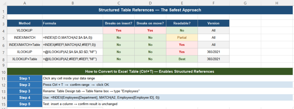
Converting your data range to an Excel Table (Ctrl+T) is the single most effective structural improvement you can make. It enables column-name references that are immune to reordering.
How to convert:
- Click any cell inside your data range.
- Press Ctrl + T.
- Confirm the range and click OK.
- In the Table Design tab, rename the table (for example, “Employees”).
- Update your formulas to use
Employees[Column Name]references.
After this, inserting or moving columns within the table does not break any formula that uses structured references.
Comparison: VLOOKUP vs INDEX/MATCH vs XLOOKUP
| Feature | VLOOKUP | INDEX/MATCH | XLOOKUP |
|---|---|---|---|
| Breaks when columns are inserted | Yes — silently | No | No |
| Breaks when columns are moved | Yes | No (with column refs) | No |
| Can look left | No | Yes | Yes |
| Supports table (structured) references | Partial | Yes | Yes |
| Default match type | Approximate (dangerous) | Exact (when 0 is set) | Exact |
| Built-in “not found” value | No — use IFERROR | No — use IFERROR | Yes (4th argument) |
| Multiple match criteria | No | Yes (array formula) | Yes (with &) |
| Excel version required | All | All | 365 / 2021+ |
Step-by-Step Migration Plan
Replacing VLOOKUP in an existing workbook does not need to be done all at once. This sequence keeps the workbook stable throughout the process.
Step 1 — Find all VLOOKUP formulas
Press Ctrl + F, set “Look in” to Formulas, and search for VLOOKUP. Note which sheets and how many cells are affected.
Step 2 — Identify the highest-risk formulas first
Prioritize formulas that reference tables modified by multiple people, or tables that are refreshed from external sources. These are most likely to experience column changes.
Step 3 — Work on a copy
Duplicate the sheet before making changes. This gives you a rollback point if anything goes wrong.
Step 4 — Replace one formula and verify
Replace one VLOOKUP with its INDEX/MATCH or XLOOKUP equivalent. Confirm both return the same result before proceeding.
Step 5 — Test structural resilience
After replacing a formula, insert a temporary column into the lookup table, confirm the result did not change, then delete the test column. This is the only way to verify the formula is truly robust.
Step 6 — Convert the table to an Excel Table
Once the formulas are replaced, convert the data range to an Excel Table (Ctrl+T) and update references to use column names. This protects against all future column changes automatically.
Quick Checklist
- VLOOKUP uses a hardcoded column index that breaks when columns are inserted, deleted, or moved
- The error is silent — no error message, just wrong values
- INDEX/MATCH references columns directly and is safe in all Excel versions
- XLOOKUP is the cleanest replacement for Excel 365 and Excel 2021
- Excel Table structured references (Ctrl+T) make formulas immune to column reordering
- Always use exact match:
0in MATCH,FALSEin VLOOKUP - Test resilience by inserting a test column and verifying results do not change
Frequently Asked Questions
Why does VLOOKUP return the wrong value after I insert a column?
VLOOKUP identifies the return column by its position number — for example, “return the 3rd column from the left of the range.” When a column is inserted, all columns to the right shift by one position. The number 3 now points to a different column than before, and Excel has no way to detect this. The formula continues to run without errors, but returns data from the wrong column.
Does INDEX/MATCH break when columns are inserted?
Not when written correctly. INDEX/MATCH references columns by their letter or by a table column name, not by a positional integer. When a column is inserted, Excel automatically updates column letter references (for example, D:D becomes E:E if a column is inserted before D). If you use Excel Table structured references like Employees[Department], the reference always points to the Department column regardless of its position.
Can I use VLOOKUP safely if I promise not to insert columns?
In a single-user workbook with a completely stable structure, VLOOKUP is technically safe. In any shared workbook, any workbook connected to an external data source, or any workbook that may be modified in the future, the risk is too high. The cost of switching to INDEX/MATCH is low; the cost of a silent wrong-value error in a report is high.
What is the MATCH 0 argument for?
The third argument in MATCH controls the match type. Setting it to 0 forces exact match — it only returns a result when the lookup value is found exactly. Omitting it or setting it to 1 uses approximate match, which assumes data is sorted in ascending order and can return wrong results when it is not. Always use 0 for lookup tables.
Is XLOOKUP available in Excel 2019?
No. XLOOKUP is only available in Excel for Microsoft 365, Excel 2021, Excel for the web, and Excel on mobile. It is not available in Excel 2019, 2016, or earlier versions. If your workbook needs to be compatible with Excel 2019 or older, use INDEX/MATCH instead, which works in all Excel versions.