You build a VLOOKUP formula, it works perfectly — and then, weeks later, the numbers are quietly wrong. No error. No warning. Just bad data.
This is one of the most dangerous failure modes in Excel: a formula that looks correct but returns the wrong result. If you rely on that number to make a decision, you’ll never know something went wrong.
This post explains exactly why VLOOKUP breaks in real workbooks, shows you three reliable alternatives, and gives you a step-by-step migration plan you can use today.
What the Problem Looks Like
Here is the most common scenario:
- You write
=VLOOKUP(A2, B:F, 4, FALSE)to pull a price from column 5 of a table. - It works correctly for weeks.
- A colleague inserts a new “Notes” column between columns C and D to add comments.
- Your formula still runs without errors — but now returns the wrong column’s data.
- Nobody notices until a report is already distributed.
This is not a bug. Excel did exactly what the formula asked. The problem is what the formula asks for.
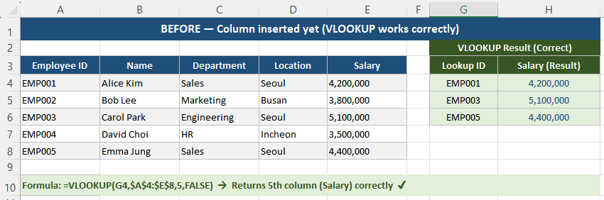
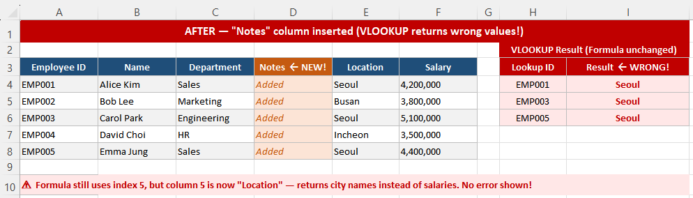
After inserting a column, VLOOKUP silently shifts to the wrong data — no error is shown.
Why VLOOKUP Breaks — 4 Root Causes
1. VLOOKUP is position-based, not name-based
The third argument in VLOOKUP is a column index number — a hardcoded integer like 4. It means “return whatever is in the 4th column of this range,” not “return the column named Price.”
Every time the physical structure of your table changes — a column added, deleted, or reordered — that integer now points somewhere different. Excel has no way to know your intent. It just counts columns from the left.
2. It can only look to the right
VLOOKUP requires the lookup column to be the leftmost column in the range. If you need to look up a value using a column that isn’t on the far left, you cannot use VLOOKUP without restructuring your data.
This constraint forces bad workarounds: copy-pasting columns into different positions, creating hidden helper columns, or duplicating data. Each workaround adds maintenance risk.
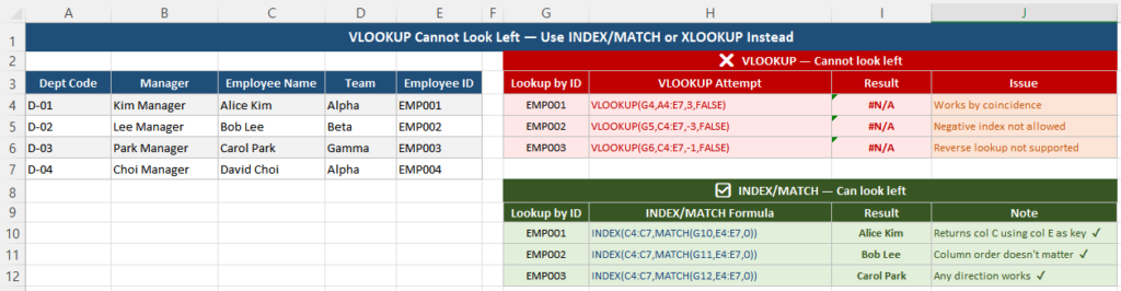
VLOOKUP can only look right. If your lookup key is not in the first column of your range, you need a workaround.
3. Exact match is not the default
When you omit the fourth argument — or set it to TRUE — VLOOKUP uses approximate match. This means it finds the largest value that is less than or equal to the lookup value, assuming data is sorted ascending.
If your data is not perfectly sorted, or if new rows are added, approximate match returns a plausible-looking but wrong result. The most dangerous type of error is one that looks believable.
The safe default is always FALSE (exact match), but many formulas inherited from others, or written quickly, leave this out.
4. VLOOKUP assumes static, controlled data
VLOOKUP was designed in an era of stable, single-user spreadsheets. Modern workbooks are shared across teams, refreshed from Power Query, expanded monthly, and restructured regularly. VLOOKUP’s rigid positional logic does not adapt to any of this automatically.
How to Fix It: 3 Reliable Alternatives
Option A — XLOOKUP (recommended for Excel 365 / 2021+)
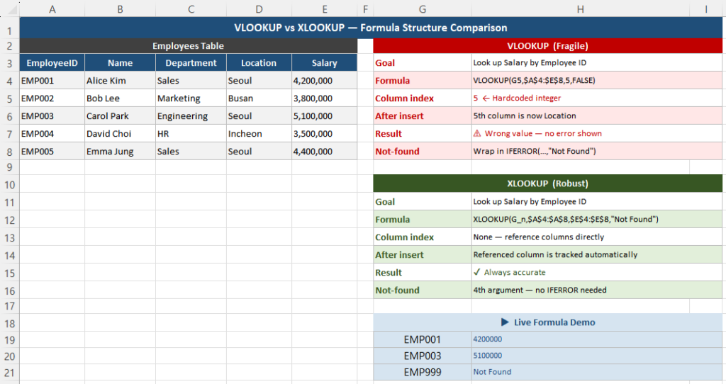
XLOOKUP is the direct replacement for VLOOKUP. Instead of a column index number, you specify the exact column you want to return.
VLOOKUP (fragile):
=VLOOKUP(A2, B:F, 4, FALSE)XLOOKUP (robust):
=XLOOKUP(A2, B:B, E:E, "Not Found")Key differences:
- No column index number — columns can move freely
- Can look left, right, or across sheets
- Has a built-in “not found” argument so missing results are visible, not silent
- Default is exact match — no accidental approximate matches
With structured table references (best practice):
=XLOOKUP([@EmployeeID], Employees[EmployeeID], Employees[Department], "Not Found")Now if the Department column moves within the Employees table, the formula updates automatically.
Option B — INDEX/MATCH (compatible with all Excel versions)
XLOOKUP references columns by name, not position. Inserting or moving a column does not break the result.
If you are on Excel 2016, 2019, or need compatibility with older files, INDEX/MATCH is the standard robust alternative to VLOOKUP.
Basic syntax:
=INDEX(E:E, MATCH(A2, B:B, 0))How it works:
MATCH(A2, B:B, 0)finds the row number where A2 appears in column B. The0means exact match.INDEX(E:E, ...)returns the value at that row number from column E.
Because both functions reference columns directly, moving columns around does not change results.
Looking left (not possible with VLOOKUP):
=INDEX(A:A, MATCH(D2, E:E, 0))This returns a value from column A based on a match in column E — impossible with VLOOKUP without restructuring the table.
Option C — XLOOKUP with multiple criteria
When you need to match on two or more conditions, XLOOKUP supports this cleanly using the & concatenation operator:
=XLOOKUP(A2&B2, C:C&D:D, E:E, "Not Found")This matches rows where both column C equals A2 and column D equals B2 — a common requirement that previously needed complex array formulas.
Step-by-Step Migration Plan
Migrating an existing workbook from VLOOKUP to XLOOKUP or INDEX/MATCH does not have to be risky. Follow this sequence:
Step 1 — Audit how many VLOOKUP formulas you have
Press Ctrl + F, select “Look in: Formulas,” and search for VLOOKUP. Note how many cells use it and which sheets they are on.
Step 2 — Identify which are highest risk
Formulas on sheets that are shared, refreshed from external sources, or frequently edited are highest priority. Static reference sheets with no team access are lower priority.
Step 3 — Replace one formula at a time, in a copy first
Duplicate the sheet or save a backup copy. Replace one VLOOKUP with its XLOOKUP equivalent, then verify the results match before proceeding.
Step 4 — Convert plain ranges to Excel Tables
Select any plain data range and press Ctrl + T to convert it to an Excel Table. This enables structured references like Employees[EmployeeID] that are immune to column reordering.
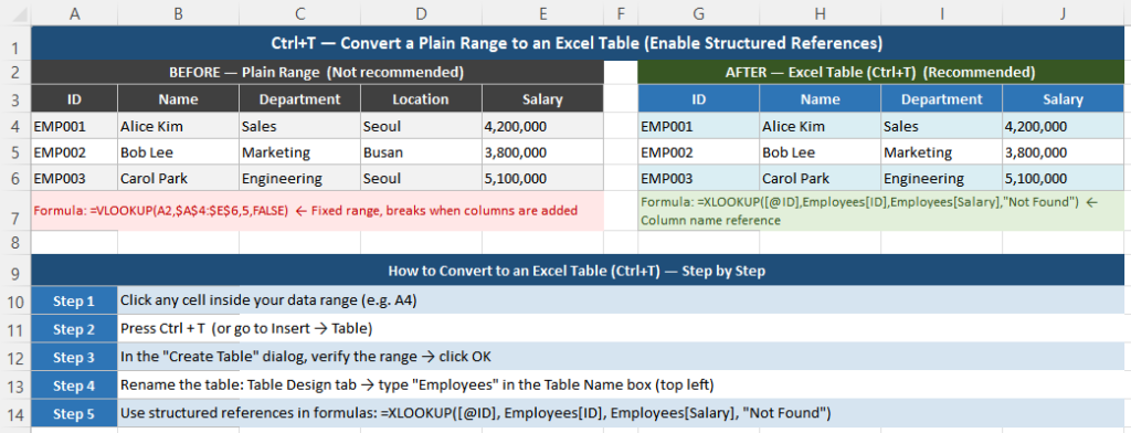
Converting to an Excel Table enables structured references that do not break when columns move.
Step 5 — Sanity check after each change
After replacing each VLOOKUP, insert a test column next to the result, then delete it. Confirm the formula result did not change. Repeat for every replaced formula.
VLOOKUP vs XLOOKUP vs INDEX/MATCH — Side-by-Side
| Feature | VLOOKUP | XLOOKUP | INDEX/MATCH |
|---|---|---|---|
| Column position matters? | Yes — breaks if columns move | No | No |
| Can look left? | No | Yes | Yes |
| Default match type | Approximate (dangerous) | Exact (safe) | Exact (when 0 is set) |
| Built-in “not found” value | No (use IFERROR wrapper) | Yes (4th argument) | No (use IFERROR wrapper) |
| Multiple criteria | Not supported | Yes (with &) | Yes (array formula) |
| Excel version required | All versions | Excel 365 / 2021+ | All versions |
| Works with structured tables | Partial | Full | Full |
| Silent wrong results possible? | Yes — high risk | No — visible failure | No — returns error or IFERROR message |
Better Practices for Long-Term Stability
Always use exact match explicitly
Whether you keep VLOOKUP or migrate to INDEX/MATCH, always specify exact match explicitly. In VLOOKUP, set the fourth argument to FALSE. In MATCH, set the third argument to 0. Never leave it to the default.
Use named ranges or table references instead of column letters
A formula like =XLOOKUP(A2, PriceList[SKU], PriceList[Price]) is self-documenting and survives structural changes. A formula like =XLOOKUP(A2, B:B, D:D) breaks if column C is inserted.
Make failures visible, not silent
Always add a “not found” fallback. For XLOOKUP, use the fourth argument. For INDEX/MATCH, wrap in IFERROR:
=IFERROR(INDEX(E:E, MATCH(A2, B:B, 0)), "Not Found")A cell showing “Not Found” is immediately visible. A cell showing a plausible but wrong number is not.
Keep lookup logic out of deeply nested formulas
When a lookup is buried inside an IF, SUMIF, or other function, debugging a wrong result becomes much harder. Keep lookups as standalone cells when possible, and reference those cells in downstream formulas.
For large datasets: use bounded ranges, not full columns
Referencing entire columns like A:A is convenient but forces Excel to scan up to 1,048,576 rows every time. For large models, use bounded ranges (A2:A10000) or table column references, both of which recalculate faster.
Quick Checklist
- VLOOKUP returns the wrong column when columns are inserted, deleted, or moved
- Approximate match (the default) returns wrong rows when data is unsorted or changes
- VLOOKUP cannot look left without restructuring the table
- XLOOKUP is the best replacement for Excel 365 / 2021 — no column index, exact match by default, built-in “not found”
- INDEX/MATCH is the best replacement for older Excel versions
- Convert data ranges to Excel Tables (Ctrl+T) for structured references that survive column changes
- Always test after migration: insert and delete a column, then verify results did not change
Frequently Asked Questions
Why does VLOOKUP return the wrong value after I insert a column?
VLOOKUP identifies the return column by its position number (e.g., “the 4th column from the left”). When you insert a column, all columns to the right shift by one position, so the number now points to a different column. Excel does not detect this as an error — it simply returns whatever is in that new position.
Is XLOOKUP available in all versions of Excel?
XLOOKUP is available in Excel for Microsoft 365, Excel 2021, Excel for the web, and Excel on mobile. It is not available in Excel 2019, 2016, or earlier. If you need compatibility with older versions, use INDEX/MATCH instead, which works in all Excel versions back to Excel 2003.
What is the difference between VLOOKUP exact match and approximate match?
Exact match (FALSE or 0) returns a result only if the lookup value is found exactly. If the value is missing, it returns an error. Approximate match (TRUE or 1, the default) returns the largest value less than or equal to the lookup value, assuming data is sorted in ascending order. Approximate match is appropriate for range lookups (such as tax brackets) but is dangerous for ID or name lookups, where it can return the wrong row silently.
Can VLOOKUP look to the left?
No. VLOOKUP requires the lookup column to be the leftmost column in the specified range. If you need to return a value that is to the left of the lookup column, you must use XLOOKUP or INDEX/MATCH, both of which can look in any direction.
Should I replace all my VLOOKUP formulas with XLOOKUP?
If your workbook is used only in Excel 365 or Excel 2021, yes — XLOOKUP is more robust, easier to read, and less prone to silent errors. If the file is shared with people using Excel 2019 or older, use INDEX/MATCH as a compatible alternative. Migrate high-risk formulas first: those on shared sheets, those pulling from frequently edited tables, and those where a wrong result would not be immediately obvious.
Closing
VLOOKUP is not wrong — it was the right tool for a different era. The workbooks we use today are shared, dynamically updated, and regularly restructured. VLOOKUP’s position-based logic cannot keep up with that safely.
XLOOKUP and INDEX/MATCH both express intent rather than position. They fail visibly rather than silently. And they require no special skills to use — just a change in the formulas you write.
If you have one VLOOKUP formula in a critical report, migrate it this week. If you have dozens, start with the highest-risk sheet and work outward. The checklist above gives you a repeatable process for each one.
Related articles on this site: