You write a formula once. It is correct on that first row, so you copy it down across the rest of the column — a routine, almost reflexive step in building any report. The numbers that come back no longer make sense: some rows look too high, others too low, and the totals at the bottom no longer match what a manual check would suggest.
This is not a bug, and it is not random. Excel is doing exactly what it was designed to do when you copy a formula — it is just that what Excel assumes you want and what your business logic actually requires are not always the same thing. This post walks through why this happens, fixes a realistic sales-commission scenario where it goes wrong, and gives you a structural habit that prevents it from recurring.
What Copying a Formula Actually Does
When you copy a formula to a new location, Excel’s default assumption is that every cell reference inside it should shift relative to the new position — this is called a relative reference. Copying a formula down moves its row references; copying it across moves its column references. Excel applies this automatically, on every copy, regardless of whether that is actually what your formula needs.
Four Reasons This Keeps Happening
1. Excel adjusts references by default, with no exceptions assumed
Relative reference behavior is the baseline for every formula you write, unless you explicitly tell Excel otherwise. There is no setting that makes Excel ask “should this one stay fixed?” — it simply shifts everything consistently, every time.
2. Not all references should move, but Excel cannot know which ones
Real-world formulas frequently mix two different kinds of inputs: values that genuinely change per row, like a sales amount, and values that must stay constant across every row, like a commission rate or a tax percentage. Excel has no way to infer this distinction from the formula’s logic alone — it relies entirely on you to mark which references are fixed.
3. The resulting errors look exactly like valid numbers
This is what makes the problem genuinely dangerous rather than merely annoying. When a reference shifts to an unintended cell, the formula still calculates successfully and the cell still displays a normal-looking number. No error appears, because as far as Excel is concerned, nothing went wrong — the formula referenced a valid cell and returned a valid result.
4. The error compounds as the formula spreads further
The more rows or columns a flawed formula gets copied across, the harder the original mistake becomes to trace, and the more inconsistent the visible results become from row to row. By the time someone notices that totals do not add up, the root cause is often buried under dozens or hundreds of copies of the same shifted formula.
Scenario: Sales Commission Calculation
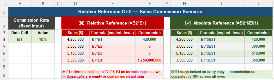
Consider a commission report: column B holds the sales amount for each row, cell E1 holds a fixed commission rate, and column C is meant to calculate the resulting commission for each row. The formula in C2 is:
=B2*E1This is correct for the first row — B2 multiplied by the rate in E1 produces the right commission value. Copying this formula down the rest of column C produces drift: the second row’s formula becomes =B3*E2, the third becomes =B4*E3, and so on. The sales amount reference correctly tracks down with each row, but the commission rate reference is also shifting down, away from E1, into cells that are empty or contain unrelated values entirely.
Fixing It With Absolute References
Step 1 — Identify which reference must never move. Before copying any formula, ask explicitly: if this formula is copied elsewhere, which reference should change, and which one must stay exactly where it is? In this scenario, the sales amount (B2) should move with each row; the commission rate (E1) must not move at all.
Step 2 — Lock the fixed reference with dollar signs. An absolute reference, written with dollar signs before both the column letter and row number, tells Excel explicitly never to shift that reference during a copy:
=B2*$E$1Now B2 still adjusts normally as the formula is copied down — becoming B3, B4, B5 — while $E$1 stays locked on the exact same cell in every single copy, regardless of how far the formula spreads.
Step 3 — Copy the corrected formula and check multiple rows. After applying the fix, copy the formula down again and inspect several rows directly. Confirm that the commission rate is now identical across all of them, and that the resulting commission values align with what a manual calculation would produce.
Step 4 — Inspect, don’t just glance. Click on a few of the copied formulas individually and look at exactly which part of each reference changed and which part stayed fixed. A healthy pattern shows row references moving where expected and the locked reference staying perfectly still everywhere. If you see the locked reference drifting in even one cell, stop and investigate immediately rather than continuing to copy further.
Relative, Absolute, and Mixed References
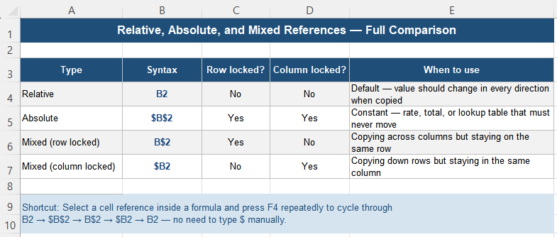
Excel supports four distinct referencing behaviors, and choosing the right one for each part of a formula is the entire solution to this problem:
| Type | Syntax | Row locked? | Column locked? | When to use |
|---|---|---|---|---|
| Relative | B2 | No | No | Default — the value should change in every direction when copied |
| Absolute | $B$2 | Yes | Yes | A constant — rate, total, or lookup table that must never move |
| Mixed (row locked) | B$2 | Yes | No | Copying across columns while staying on the same row |
| Mixed (column locked) | $B2 | No | Yes | Copying down rows while staying in the same column |
A practical shortcut: select a cell reference inside a formula in the formula bar and press F4 repeatedly. Excel cycles through all four forms automatically — B2 → $B$2 → B$2 → $B2 → back to B2 — without needing to type dollar signs manually.
Sanity Check After Copying
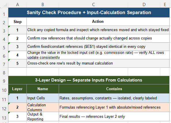
After locking the appropriate references and copying the formula, confirm the fix with three checks:
- Individual row results make sense — spot-check several rows and confirm each commission value is proportionate to its sales amount
- Totals align with a manual check — sum the commission column and compare against an independent calculation
- Changing the locked input updates everything consistently — change the value in the rate cell (E1) and confirm every row’s commission updates accordingly, in proportion, with no row left behind or calculated differently
If all three hold, the reference logic in the formula is structurally sound, not just accidentally correct for the rows you happened to check.
Decide Reference Behavior Before You Copy
Absolute references are not a workaround or a trick for advanced users — they are a basic design tool that should be considered before a formula is ever copied, not after something looks wrong. Before spreading any formula across rows or columns, explicitly ask which of its inputs are variable and which are constants. Deciding this upfront prevents the cascading drift described in this scenario from ever occurring in the first place.
Stable Excel models typically separate three layers: input cells holding rates and assumptions, calculation columns that reference those inputs with the correct mix of absolute and relative references, and an output or reporting layer built on top of the calculations. When inputs are isolated this way, it becomes immediately obvious which references need to be locked, and the resulting formulas are far easier for anyone to audit later.
Because a formula with a shifted reference still returns a number that looks entirely plausible, visual inspection alone is not a reliable way to catch this class of error — a quick glance at the results will not reveal that a reference moved somewhere it should not have. Reference correctness needs to be verified structurally, using the sanity check steps above, not assumed from how the output appears. For large tables specifically, build and validate the formula logic on a small sample first, lock references deliberately at that stage, and only then copy the formula across the full dataset — fixing a reference mistake after it has already propagated across thousands of rows is far more expensive than preventing it from the start.
Quick Checklist
- Excel shifts all references by default when a formula is copied — this is relative reference behavior
- Identify explicitly which references should move and which must stay fixed before copying
- Use $B$2 (absolute) to lock both the row and column of a reference completely
- Use B$2 or $B2 (mixed) when only one dimension needs to stay fixed
- Press F4 to cycle through reference types quickly without typing dollar signs manually
- A formula with a shifted reference still returns a normal-looking number — there is no visible error
- Verify correctness by changing a locked input and confirming every dependent row updates consistently
- Separate input cells from calculation formulas to make locking the right references easier and more obvious
Frequently Asked Questions
Why do my formula results change when I copy a formula down a column?
By default, Excel uses relative references, which shift automatically based on where a formula is copied. If your formula references a cell that should stay constant — such as a fixed rate or a lookup total — without locking it as an absolute reference, that reference will drift to a different, often empty or unrelated, cell in each copied row. Add dollar signs before the column letter and row number, such as $E$1, to lock that specific reference in place.
What is the difference between a relative and an absolute reference in Excel?
A relative reference, written without dollar signs (such as B2), shifts automatically to match the new position whenever the formula is copied. An absolute reference, written with dollar signs before both the column and row (such as $B$2), stays locked on that exact cell no matter where the formula is copied. Use relative references for values that should vary by row or column, and absolute references for constants that must remain the same everywhere.
How do I quickly add dollar signs to a cell reference in Excel?
Click on the cell reference within the formula bar, then press the F4 key. Excel cycles through all four reference types in sequence: relative (B2), fully absolute ($B$2), row-locked mixed (B$2), and column-locked mixed ($B2), pressing F4 again returns to relative. This is faster than manually typing dollar signs, especially when adjusting several references in a longer formula.
Why didn’t Excel show an error if my formula reference was wrong after copying?
A shifted reference still points to a valid cell — it is simply not the cell you intended. Because the cell exists and contains some value (or is empty, which Excel treats as zero in arithmetic), the formula calculates successfully and displays a normal-looking number. Excel has no way to know that the reference was unintentional, so no error is raised. This is exactly why this class of mistake is dangerous: the output looks plausible even when it is wrong.
What is a mixed reference and when should I use one?
A mixed reference locks only one dimension — either the row or the column — while leaving the other free to shift. B$2 locks the row but lets the column move, useful when copying a formula across columns while it needs to stay anchored to a specific row, such as a header value. $B2 locks the column but lets the row move, useful when copying down rows while staying anchored to a specific column. These are especially common in two-dimensional lookup tables and cross-tabulated reports.