You click Refresh. Excel responds instantly, as if the operation completed successfully. The numbers in the Pivot Table do not move at all. New rows from this month’s data are missing, the totals match last month exactly, and the report looks frozen in time despite the refresh having clearly run.
Excel is not ignoring the click. The Pivot Table is refreshing exactly what it was told to refresh — the problem is that what it was told often does not match what you actually need refreshed. This post walks through why Pivot Tables behave this way, fixes a realistic monthly sales scenario where new data goes missing, and shows you the structural change that prevents the problem from recurring every month.
What Refresh Actually Does
A Pivot Table is not a live window into your data. When created, Excel takes a snapshot of the source range and stores it separately in something called a Pivot Cache. Every calculation you see — sums, counts, groupings — is computed from this cache, not by reading the source cells directly each time.
Clicking Refresh updates this cache — but only within the boundaries that were defined when the Pivot Table was created or last configured. If new data exists outside those original boundaries, Refresh has no way to discover it, because it is not scanning the worksheet freshly each time; it is re-reading a defined range that may no longer match where your data actually lives.
Four Reasons Refresh Looks Like It Failed
1. Pivot Tables run on a cache, not live cells
The cache is a snapshot, refreshed on demand, but only within its defined extent. This is fundamentally different from a formula like SUMIFS, which always reads the current state of whatever range it references.
2. The source range does not expand on its own
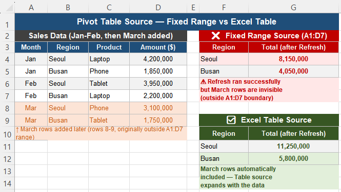
If a Pivot Table’s source is defined as a fixed range — for example A1:D100 — and new rows are added starting at row 101, Excel treats row 100 as the deliberate, intended boundary of the data. Refresh runs successfully and reports no error, because nothing within the defined range actually changed incorrectly; the new rows are simply invisible to it.
3. The underlying data may not have genuinely changed
In some workflows, data is overwritten via copy-paste with values that happen to be identical, formulas recalculate but settle on the same numbers as before, or external links still point to an old file version. From the Pivot Table’s perspective, nothing changed — so naturally, the result looks the same after Refresh, because it is the same.
4. Multiple Pivot Tables can share one cache
If several Pivot Tables are built from the same source data, they may share a single underlying Pivot Cache. Refreshing one does not always behave the way you would expect relative to the others, which can make debugging confusing — it can feel like Excel is selectively ignoring your refresh action.
Scenario: A Monthly Sales Report
Consider a monthly sales report where new rows are appended to the bottom of a data sheet each month, and a Pivot Table summarizes total sales by region. After this month’s data is added and Refresh is clicked, the latest month’s rows are missing entirely from the regional totals.
Fixing It Step by Step
Step 1 — Check the Pivot Table’s actual source. Click anywhere inside the Pivot Table, then check its data source (PivotTable Analyze tab → Change Data Source, or check the Name Box reference). If the source is a fixed cell range ending at a specific row, that boundary is very likely the root cause.
Step 2 — Convert the source data into an Excel Table. Select the raw data range and press Ctrl + T. Excel Tables expand automatically as new rows are added directly below them, and any Pivot Table linked to a Table — rather than a fixed range — will always see those new rows without any manual range adjustment.
Step 3 — Rebuild or repoint the Pivot Table. If the Pivot Table predates the Table’s creation, update its source to point to the new Table name via Change Data Source, or rebuild the Pivot Table once from scratch using the Table as the source. After this change, adding rows in the future updates the Pivot Table automatically on the next Refresh — no further manual maintenance required.
Step 4 — Verify the data genuinely changed. Before assuming the Pivot Table itself is broken, check the raw data directly: confirm new rows actually contain different values, and that any formulas feeding the source data updated correctly. A refresh can only ever reflect a real change — it cannot surface a change that did not actually happen.
Sanity Check: The Test Row Method
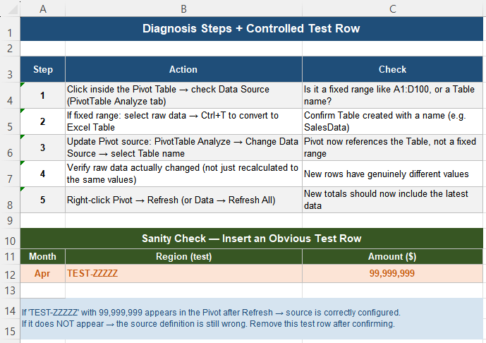
To remove all ambiguity about whether the fix worked, add one deliberately obvious test row to the source data — a unique region name nothing else uses, paired with a large, unmistakable number. Refresh the Pivot Table.
- If the test row appears in the results, the source structure is now correct.
- If it does not appear, the source definition is still pointing somewhere other than where you expect — recheck the Change Data Source dialog.
Remove the test row once the structure is confirmed working correctly.
The Shared Cache Trap
If multiple Pivot Tables are built from the same underlying source, they may silently share one Pivot Cache. This can produce a confusing symptom: refreshing Pivot Table A does not seem to update Pivot Table B, even though both draw from what looks like the same data.
The reliable fix is to use Data → Refresh All rather than refreshing a single Pivot Table individually, which ensures every cache connected to the workbook updates together rather than relying on assumptions about which Pivot Tables share which cache.
Design Sources for Growth From the Start
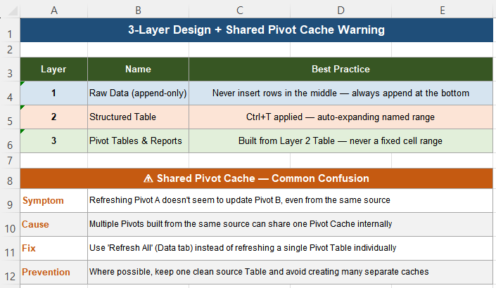
Pivot Table refresh problems are almost always design issues discovered after the fact, not mistakes in how the button was clicked. A stable structure follows three layers:
| Layer | Name | Best practice |
|---|---|---|
| 1 | Raw Data (append-only) | Never insert new rows in the middle — always append at the bottom |
| 2 | Structured Table | Converted with Ctrl+T — an auto-expanding named range |
| 3 | Pivot Tables & Reports | Built from the Layer 2 Table — never from a fixed cell range |
If data is expected to grow over time — which describes the vast majority of recurring business reports — never use a fixed range as the Pivot Table source. An Excel Table or another dynamic source turns Refresh into a reliable, predictable operation instead of something that needs re-verifying every month. Be especially careful with copy-paste workflows: if data is pasted directly over existing rows rather than appended below them, Pivot Tables can show no visible change even though the cache technically updated, simply because the new values happen to be similar to the old ones. Appending rows is the safer pattern whenever reports depend on refresh behavior. For large Pivot-based reporting setups, maintain one clean source Table, avoid rebuilding Pivot Tables repeatedly from scratch, and refresh intentionally rather than constantly — this keeps both performance and your own understanding of cache state manageable.
Quick Checklist
- Pivot Tables calculate from a cached snapshot, not live cells — Refresh updates the cache only within its defined boundary
- A fixed-range source does not expand when new rows are added below it
- Convert source data to an Excel Table (Ctrl+T) so the boundary always matches the actual data
- Verify the underlying data genuinely changed before assuming the Pivot Table is broken
- Use a test row with an obvious unique value to confirm the source is correctly configured
- Multiple Pivot Tables sharing one source may share one cache — use Refresh All, not individual refreshes
- Append new data at the bottom rather than overwriting existing rows when reports depend on refresh
- Design Pivot sources for growth from the start — never use a fixed range for data expected to expand
Frequently Asked Questions
Why doesn’t my Pivot Table show new rows after I click Refresh?
The most common cause is that the Pivot Table’s source is defined as a fixed cell range, such as A1:D100, and the new rows were added below that boundary. Refresh updates the Pivot Cache only within the range that was originally defined, so rows outside that boundary are invisible to it even though the refresh itself completes successfully. Convert the source data into an Excel Table with Ctrl+T, which expands automatically as rows are added, and update the Pivot Table to reference the Table instead of the fixed range.
What is a Pivot Cache and why does it matter?
A Pivot Cache is a snapshot of the source data that Excel stores separately when a Pivot Table is created. All Pivot Table calculations run against this cache, not against the live worksheet cells directly. Refreshing updates the cache, but only for the range or Table that the Pivot Table is configured to read from. Understanding this explains why Refresh can complete successfully while still appearing to show stale results — the cache itself was never told to look beyond its original boundary.
How do I make a Pivot Table automatically include new rows in the future?
Convert the source data range into an Excel Table using Ctrl+T, then point the Pivot Table’s data source to that Table by name rather than to a fixed cell range. Excel Tables expand automatically whenever new rows are added directly below them, so any Pivot Table referencing the Table will pick up new data on the next Refresh, with no manual range adjustment ever required again.
Why does refreshing one Pivot Table not update another one built from the same data?
Multiple Pivot Tables created from the same source data can share a single underlying Pivot Cache, which can lead to inconsistent-looking refresh behavior between them. Use Data → Refresh All instead of refreshing each Pivot Table individually — this ensures every cache connected to the workbook is updated together, removing the ambiguity around which Pivot Tables share which cache.
How can I quickly verify whether my Pivot Table source is configured correctly?
Add one deliberately obvious test row to the source data — for example, a unique label like “TEST-ZZZZZ” paired with a very large, unmistakable number — then click Refresh. If the test row appears in the Pivot Table results, the source is correctly configured to pick up new data. If it does not appear, the source definition still needs to be corrected. Remove the test row once you have confirmed the result.