One formula returns #N/A. Then every formula that depends on it also returns #N/A. By the time you open the report, half the cells show errors and the underlying cause is buried somewhere in a chain of dependent formulas.
Excel errors are not accidents — they are signals. The problem is not that the errors exist, but that they appear in the wrong place, propagate further than intended, and make reports unreadable before anyone can diagnose the root cause.
This post explains what each common error means, why errors spread, and how to stop propagation at the right layer without hiding problems that should remain visible.
Why Errors Spread Through a Workbook
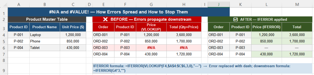
Excel propagates errors by design. When a formula returns an error value like #N/A or #VALUE!, any formula that references that cell also returns an error — regardless of what the downstream formula is trying to do.
A single #N/A in a VLOOKUP column cascades into:
- Every calculation that multiplies or divides by that cell
- Every SUM or AVERAGE that includes the range
- Every chart data series connected to that range
- Every Pivot Table field drawing from that column
This is intentional behavior. Excel assumes that an error in a source cell means the downstream result is also unreliable. The problem in practice is that some errors are expected — a lookup that finds no match for a new product is not a formula failure, it is a data condition — and the error should be handled at a specific point rather than allowed to cascade.
What Each Error Actually Means
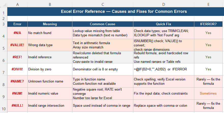
#N/A — No match found
Returned by lookup functions (VLOOKUP, XLOOKUP, MATCH, INDEX/MATCH) when the lookup value does not exist in the lookup range. Common causes: the value is genuinely missing, or a data type mismatch means a number in one column is stored as text in the other.
#VALUE! — Wrong data type
Returned when a formula tries to perform arithmetic on a text value, or when two arrays in a formula have incompatible sizes. If a cell that should contain a number contains text like “N/A” or a space, any formula that performs arithmetic on it returns #VALUE!.
#REF! — Invalid cell reference
Returned when a formula references a cell that no longer exists — most commonly because a row or column was deleted after the formula was written. Unlike other errors, #REF! almost always indicates a structural problem that should be fixed rather than suppressed.
#DIV/0! — Division by zero
Returned when a formula divides by a cell that contains zero or is empty. Common in percentage calculations and rate formulas where the denominator may not yet have data.
#NAME? — Unrecognized function name
Returned when Excel does not recognize the function name in a formula — usually a typo, or a function that exists in a newer Excel version than the one in use. This error should always be fixed at the formula level, not suppressed with IFERROR.
#NUM! — Invalid numeric result
Returned when a formula produces a number that Excel cannot represent — for example, a square root of a negative number, or an iterative function like RATE or IRR that fails to converge.
How IFERROR Stops Propagation
IFERROR wraps any formula and replaces its output with a specified value whenever an error occurs:
=IFERROR(formula, value_if_error)Basic example — VLOOKUP with blank fallback:
=IFERROR(VLOOKUP(A2, PriceList, 2, FALSE), "")If VLOOKUP finds no match, the cell shows blank instead of #N/A. Downstream formulas that reference this cell receive a blank, not an error — propagation stops here.
Apply at the right level:
-- Price column (source):
=IFERROR(VLOOKUP(A2, PriceList, 2, FALSE), "")

-- Total column (downstream):
=IF(B2="", "", B2 * C2)
The IF in the Total formula skips calculation when the price is blank, producing a clean result instead of another error or an unexpected zero.
For cases where you want to suppress only #N/A (not all errors), use IFNA instead:
=IFNA(VLOOKUP(A2, PriceList, 2, FALSE), "")IFNA is more precise — it only catches #N/A errors. If VLOOKUP returns #VALUE! due to a data problem, IFNA lets that error through, which helps during debugging.
Choosing Between Blank and Zero
The choice of fallback value in IFERROR matters more than it appears:
| Use blank (“”) | Use 0 |
|---|---|
| Value is informational (name, label, category) | Value feeds arithmetic (SUM, AVERAGE, charts) |
| Zero would distort averages | Missing data genuinely means no contribution |
| Chart should show a gap, not a zero data point | Chart should plot zero for missing periods |
| Pivot Table should show an empty cell | Pivot Table should count missing as zero |
The most common mistake is defaulting to 0 everywhere. A SUM over a range with zeros and blanks produces the same result, but an AVERAGE does not — zeros pull the average down, while blanks are ignored. Using zero as the fallback in a column that feeds AVERAGE calculations silently understates the average.
Where to Apply Error Handling (Three-Layer Design)
The most important principle in error handling is where you apply it. Applying IFERROR too early hides problems during development. Applying it too late lets errors reach the final report.
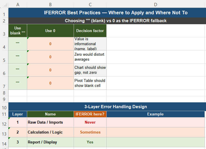
| Layer | Name | IFERROR here? | Reason |
|---|---|---|---|
| 1 | Raw Data / Imports | Never | Errors must be visible during development and validation |
| 2 | Calculation / Logic | Only for expected conditions | Suppress #N/A for known missing data; let unexpected errors through |
| 3 | Report / Display | Yes — always | Reports shown to others should never display raw error codes |
When NOT to Use IFERROR
IFERROR used carelessly creates a different problem: it hides errors that should be investigated. Four situations where suppressing errors is the wrong approach:
When the error indicates a structural problem
#REF! means a referenced cell no longer exists. #NAME? means a function name is wrong. These should be fixed, not suppressed. IFERROR applied to these errors makes the formula appear to work while masking a genuine problem.
When you are still developing the workbook
During development, visible errors are useful signals. Apply IFERROR only after the workbook is working correctly — not as a shortcut for avoiding investigation. For more on this, see Why Overusing IFERROR Breaks Excel Reports.
When the error means the data is genuinely wrong
If a product ID lookup returns #N/A because the product ID was entered incorrectly, suppressing the error lets the incorrect ID propagate silently. The error is the correct signal — it should trigger a data correction, not be hidden.
When you wrap the wrong formula
Wrapping a complex nested formula with IFERROR means any error anywhere inside it is suppressed. If the formula has multiple components, narrow the IFERROR to the specific part expected to produce errors rather than the entire expression.
Error Handling Comparison Table
| Function | Catches | Best for | Available in |
|---|---|---|---|
| IFERROR | All errors | Report-layer cleanup | All versions |
| IFNA | #N/A only | Lookup fallbacks — precise | Excel 2013+ |
| IF + ISERROR | All errors | Excel 2003 compatibility | All versions |
| IF + ISNA | #N/A only | Pre-2013 #N/A handling | All versions |
| XLOOKUP (4th arg) | #N/A only | Modern lookups — no wrapper needed | 365/2021 |
Quick Checklist
- Errors propagate to every dependent formula — one source error can fill a report
- #N/A = no match found; #VALUE! = wrong data type; #REF! = deleted reference; #DIV/0! = divide by zero
- IFERROR catches all errors; IFNA catches #N/A only — use IFNA for lookups when precision matters
- Choose blank (“”) when the value is informational; choose 0 when the value feeds arithmetic
- Apply IFERROR in the report layer, not the raw data layer
- #REF! and #NAME? should be fixed, not suppressed
- XLOOKUP’s fourth argument handles #N/A without a wrapper — preferred for Excel 365/2021
- Use IFNA during development to catch unexpected errors; switch to IFERROR only in final reports
Frequently Asked Questions
Why does one #N/A error cause my entire report to show errors?
Excel propagates error values through dependent formulas. Any formula that references a cell containing an error also returns an error. To stop propagation, apply IFERROR or IFNA at the source formula — the one that first produces the error. Once the source cell returns a blank or zero instead of an error, all downstream formulas that reference it will calculate normally.
What is the difference between IFERROR and IFNA?
IFERROR catches all error types — #N/A, #VALUE!, #REF!, #DIV/0!, and others. IFNA catches only #N/A errors. For lookup formulas where #N/A is an expected result (a product not yet in the database), IFNA is more precise — it lets other error types like #VALUE! remain visible, which helps detect unexpected problems. IFERROR is appropriate for final report displays where all errors should be suppressed for the reader.
Should I use “” or 0 as the IFERROR fallback?
Use blank (“”) when the value is informational — a name, label, or category where missing means absent. Use 0 when the value feeds arithmetic — a revenue figure, count, or quantity where missing means no contribution. The key difference is AVERAGE: a range with zeros returns a lower average than the same range with blanks, because AVERAGE ignores blank cells but counts zeros. Using 0 in a column that feeds AVERAGE calculations silently understates the result.
Why does my SUM return 0 when cells contain errors?
SUM propagates errors — if any cell in the SUM range contains an error, the entire SUM returns an error, not zero. To sum a range that may contain errors, use AGGREGATE: =AGGREGATE(9,6,A2:A100) sums while ignoring errors. Alternatively, apply IFERROR to each cell in the range to convert errors to zeros or blanks before summing.
Is it ever wrong to use IFERROR?
Yes. IFERROR is wrong when applied to errors that indicate structural problems (#REF!, #NAME?) — it hides a real issue instead of fixing it. It is also risky during development, because it masks errors that should trigger investigation. And it is wrong when applied too broadly — wrapping a large nested formula with IFERROR suppresses any error anywhere inside it, making debugging very difficult. Apply IFERROR narrowly, late in the calculation chain, and only for errors that are genuinely expected.