The value is right there — you can see it in the list. MATCH returns #N/A anyway. You double-check the spelling, verify there is no typo, and the formula still fails. Nothing about the visible content explains why.
This is one of the most frustrating troubleshooting experiences in Excel, because the answer is almost never in what you can see — it is in something invisible: a data type difference, a hidden space, or a missing argument that changes how MATCH searches. This post walks through the three root causes systematically, gives you a diagnosis checklist, and shows you the fix for each case.
What MATCH Actually Compares
MATCH does not compare what cells look like — it compares the underlying values and data types, exactly. A number and a text string that displays that number are different values to MATCH, even if they appear identical on screen. A cell containing 100 (numeric) does not match a cell containing "100" (text), and MATCH will return #N/A rather than a false positive.
Cause 1 — Data Type Mismatch
This is the most common root cause of MATCH failures on data that looks visually correct. Numbers stored as text are particularly frequent in imported data from ERP systems, CSV files, and copy-paste from web pages.
The clearest sign of a type mismatch: numbers in the lookup array are left-aligned instead of right-aligned, or a green triangle appears in the corner of cells in the array. Both indicate numbers stored as text.
Diagnosis:
=ISNUMBER(lookup_value)    ← should match =ISNUMBER(first cell in array)
=ISTEXT(A2)                ← TRUE means the value is stored as text
Fix — when the array contains text but should be numeric:
=MATCH(100, VALUE(A2:A100), 0)Fix — when the lookup is text but the array is numeric:
=MATCH(VALUE(B2), A2:A100, 0)
Cause 2 — Hidden Spaces
A cell that displays EMP001 may actually contain EMP001 or EMP001 — with a leading or trailing space that is invisible in the standard cell view. MATCH compares the full string, including any invisible characters, so the lookup fails even though the displayed content looks identical.
Diagnosis:
=LEN(A2) <> LEN(TRIM(A2))    ← TRUE means hidden spaces are present
=EXACT(lookup, array_cell)    ← FALSE confirms a character-level difference
Fix — apply TRIM to both the lookup value and the array:
=MATCH(TRIM(B2), TRIM(A2:A100), 0)For a cleaner structural fix, apply TRIM in a dedicated helper column and reference that column in MATCH instead of the raw import column. This is especially important if the same array is used in multiple lookup formulas — cleaning it once in one place is more reliable than embedding TRIM inside every formula that reads it.
Cause 3 — Wrong match_type Argument
MATCH has three possible behaviors depending on its third argument:
0— exact match: returns the position of the first cell that equals the lookup value exactly1— approximate match, ascending: assumes the array is sorted in ascending order and finds the largest value less than or equal to the lookup value-1— approximate match, descending: assumes the array is sorted in descending order
Omitting the third argument defaults to 1 (approximate match), not 0 (exact match). This default is safe only when your data is perfectly sorted in ascending order, which most real-world lookup arrays are not. If the data is unsorted and MATCH uses approximate mode, it can return the wrong row or #N/A even when an exact match exists.
Fix — always specify 0 explicitly:
=MATCH(B2, A2:A100, 0) ← explicit exact match — always safeDiagnosis Checklist
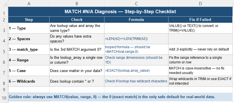
When MATCH returns #N/A unexpectedly, run through these checks in order:
| Step | Check | Formula |
|---|---|---|
| 1 — Type | Are lookup value and array the same data type? | =ISNUMBER(A2) on both |
| 2 — Spaces | Do any values have extra spaces? | =LEN(A2)<>LEN(TRIM(A2)) |
| 3 — match_type | Is the third MATCH argument explicitly 0? | Inspect the formula directly |
| 4 — Range | Is the lookup_array a single row or column? | Check the range dimensions |
| 5 — EXACT test | Does the lookup value match the array value character-for-character? | =EXACT(lookup, array_cell) |
Fix Patterns for Each Cause
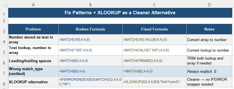
| Problem | Broken Formula | Fixed Formula |
|---|---|---|
| Number stored as text in array | =MATCH(100, A:A, 0) | =MATCH(100, VALUE(A:A), 0) |
| Text lookup, numbers in array | =MATCH("100", A:A, 0) | =MATCH(VALUE("100"), A:A, 0) |
| Leading or trailing spaces | =MATCH(B2, A:A, 0) | =MATCH(TRIM(B2), A:A, 0) |
| Missing match_type argument | =MATCH(B2, A:A) | =MATCH(B2, A:A, 0) |
XLOOKUP as a More Forgiving Alternative
For Excel 365 and Excel 2021 users, XLOOKUP is worth considering as a replacement for INDEX/MATCH patterns. XLOOKUP defaults to exact match without needing an explicit argument, accepts a not-found value directly as the fourth parameter, and can look left or right without restriction:
-- INDEX/MATCH (verbose):
=IFERROR(INDEX(B:B, MATCH(D2, A:A, 0)), "Not Found")

-- XLOOKUP (cleaner):
=XLOOKUP(D2, A:A, B:B, "Not Found")
XLOOKUP still fails on type mismatches and hidden spaces — the underlying comparison behavior is the same as MATCH. The advantage is the cleaner syntax and built-in not-found handling, not immunity to data quality problems.
Quick Checklist
- MATCH compares underlying values and types exactly — what you see on screen is not always what it compares
- A number (100) and a text string (“100”) look identical but are different types — MATCH returns #N/A
- Always specify 0 as the third MATCH argument — the default of 1 only works on sorted data
- Hidden spaces cause invisible mismatches — use TRIM on both the lookup value and the array
- Use ISNUMBER and LEN comparison to diagnose the cause before applying any fix
- Clean data in a helper column once rather than embedding VALUE or TRIM inside every MATCH formula
- XLOOKUP defaults to exact match and includes a not-found argument — a cleaner option for 365/2021
- EXACT returns TRUE only when two values match character-for-character including case — useful for diagnosing subtle differences
Frequently Asked Questions
Why does MATCH return #N/A when I can see the value in the list?
The three most common causes are a data type mismatch (a number in the lookup versus text in the array, or vice versa), hidden spaces in either the lookup value or the array values, and the match_type argument being omitted or set to 1 instead of 0. Run through each cause systematically: check ISNUMBER on both the lookup and the array, check LEN versus LEN(TRIM()) for hidden spaces, and verify the formula explicitly uses 0 as the third argument.
What does the third argument in MATCH do?
The third argument controls the match behavior. Setting it to 0 performs an exact match and works on data in any order. Setting it to 1 performs an approximate match that assumes the array is sorted in ascending order; it returns wrong results or #N/A on unsorted data. Setting it to -1 performs an approximate match assuming descending order. For real-world lookup tables that are not guaranteed to be sorted, always use 0. Omitting the argument defaults to 1, which is rarely what you want.
How do I fix MATCH when it fails because of numbers stored as text?
Wrap the array in VALUE() to convert text-stored numbers to true numbers at evaluation time: =MATCH(100, VALUE(A2:A100), 0). If the lookup value is text but the array contains true numbers, convert the lookup instead: =MATCH(VALUE(B2), A2:A100, 0). For a more permanent fix, add a helper column that applies VALUE() to the entire array once, and reference that clean column in your MATCH formula rather than the raw import column.
Is XLOOKUP better than INDEX/MATCH for avoiding these problems?
XLOOKUP offers cleaner syntax — it defaults to exact match and accepts a not-found value directly as the fourth argument, eliminating the need for an IFERROR wrapper. However, XLOOKUP is subject to the same type mismatch and hidden space failures as MATCH, because its underlying comparison logic is the same. XLOOKUP is a structural improvement over INDEX/MATCH+IFERROR, but it does not resolve data quality problems — those still need to be fixed at the source.
How can I tell if a cell contains a number or text that looks like a number?
Use =ISNUMBER(A2) — it returns TRUE for genuine numbers and FALSE for text strings, regardless of what the cell displays. You can also change the cell format to General: a true number will display as a plain numeric value, while a text string remains displayed as text. True numbers are also right-aligned by default; text values are left-aligned, which provides a quick visual scan across a column for suspected type inconsistencies.